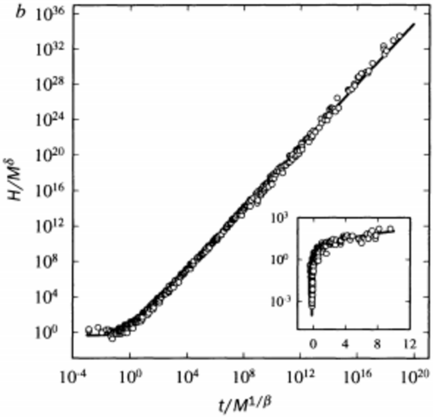
## Log-Log Plot: H/M^δ vs. t/M^(1/β) ### Overview The image presents a log-log plot showing the relationship between two dimensionless quantities: H/M^δ (y-axis) and t/M^(1/β) (x-axis). The plot exhibits a linear trend on the log-log scale, suggesting a power-law relationship. An inset plot provides a closer view of the behavior at smaller values of t/M^(1/β). ### Components/Axes * **Title:** There is no explicit title on the chart. * **Y-axis:** * Label: H/M^δ * Scale: Logarithmic (base 10) * Markers: 10^0, 10^4, 10^8, 10^12, 10^16, 10^20, 10^24, 10^28, 10^32, 10^36 * **X-axis:** * Label: t/M^(1/β) * Scale: Logarithmic (base 10) * Markers: 10^-4, 10^0, 10^4, 10^8, 10^12, 10^16, 10^20 * **Data:** * Scatter plot of data points (small circles) * Solid line representing a fit to the data * **Inset Plot:** * X-axis: 0, 4, 8, 12 (linear scale) * Y-axis: 10^-3, 10^-2, 10^-1, 10^0, 10^1 (logarithmic scale) * Data: Scatter plot of data points (small circles) and a solid line representing a fit to the data. ### Detailed Analysis * **Main Plot:** * The data points (small circles) show a clear upward trend. * The solid black line closely follows the data points, indicating a good fit. * At very small values of t/M^(1/β) (around 10^-4 to 10^0), the data points are relatively flat, suggesting a constant value of H/M^δ. * From t/M^(1/β) ≈ 10^0 to 10^20, the data points increase linearly on the log-log scale. * **Inset Plot:** * The inset plot shows the behavior of the data at small values of t/M^(1/β) on a semi-log scale. * The data points initially decrease rapidly from approximately x = 0 to x = 1. * The data points then increase rapidly from approximately x = 1 to x = 2. * The data points then level off and approach a constant value for x > 4. ### Key Observations * The main plot shows a power-law relationship between H/M^δ and t/M^(1/β) over a wide range of values. * The inset plot reveals a more complex behavior at small values of t/M^(1/β), with an initial decrease followed by an increase and then a leveling off. ### Interpretation The log-log plot suggests that H/M^δ is proportional to a power of t/M^(1/β) over a wide range. The inset plot indicates that this power-law relationship does not hold at very small values of t/M^(1/β), where other factors may be influencing the behavior of the system. The initial decrease in the inset plot could be due to some transient effect that is not captured by the power-law relationship. The leveling off at larger values in the inset suggests that the system is approaching a steady state. The plot demonstrates a scaling relationship between the variables, which is a common feature in many physical systems. The exponents δ and β likely represent critical exponents related to the underlying physics of the system.

## Chart: Log-Log Plot of H/Mδ vs. t/M¹/β ### Overview The image presents a log-log plot displaying the relationship between two variables: H/Mδ on the y-axis and t/M¹/β on the x-axis. The data is represented by a series of points connected by a line, exhibiting a generally linear trend on this log-log scale. A smaller inset plot is included in the top-right corner, showing a zoomed-in view of the data at lower values of both axes. ### Components/Axes * **X-axis Label:** t/M¹/β * **X-axis Scale:** Logarithmic, ranging from approximately 10⁻⁴ to 10²⁰. * **Y-axis Label:** H/Mδ * **Y-axis Scale:** Logarithmic, ranging from approximately 10⁰ to 10³⁶. * **Data Series:** A single data series represented by numerous points connected by a line. The points are marked with small circles. * **Inset Plot:** A smaller log-log plot in the top-right corner, with x-axis ranging from 0 to 12 and y-axis ranging from 10⁰ to 10³. * **Label:** 'b' is present at the top-left of the y-axis. ### Detailed Analysis The main plot shows a strong positive correlation between H/Mδ and t/M¹/β. The line representing the data series slopes upward, indicating that as t/M¹/β increases, H/Mδ also increases. **Main Plot Data Points (Approximate):** * At t/M¹/β ≈ 10⁻⁴, H/Mδ ≈ 10⁰ (1). * At t/M¹/β ≈ 10⁰, H/Mδ ≈ 10⁴ (10,000). * At t/M¹/β ≈ 10⁴, H/Mδ ≈ 10¹⁰ (10,000,000,000). * At t/M¹/β ≈ 10⁸, H/Mδ ≈ 10¹⁸. * At t/M¹/β ≈ 10¹², H/Mδ ≈ 10²⁶. * At t/M¹/β ≈ 10¹⁶, H/Mδ ≈ 10³². * At t/M¹/β ≈ 10²⁰, H/Mδ ≈ 10³⁶. **Inset Plot Data Points (Approximate):** * At t/M¹/β ≈ 1, H/Mδ ≈ 10¹ (10). * At t/M¹/β ≈ 4, H/Mδ ≈ 10² (100). * At t/M¹/β ≈ 8, H/Mδ ≈ 10³ (1,000). * At t/M¹/β ≈ 12, H/Mδ ≈ 10³ (1,000). The inset plot shows a more detailed view of the data at lower values, revealing a slightly curved initial segment before it appears to approach a linear trend. ### Key Observations * The relationship between H/Mδ and t/M¹/β is approximately linear on a log-log scale, suggesting a power-law relationship. * The inset plot highlights the behavior of the data at lower values, showing a possible deviation from the power-law behavior at very small t/M¹/β. * The data spans several orders of magnitude on both axes. ### Interpretation The plot suggests a scaling relationship between H and Mδ with respect to time t and parameters M and β. The approximate linearity on the log-log scale indicates that H/Mδ is proportional to t raised to some power (i.e., H/Mδ ≈ Ctⁿ, where C and n are constants). The inset plot suggests that this power-law relationship may not hold at very early times. The 'b' label near the y-axis could indicate a parameter or coefficient associated with the relationship, but its specific meaning is not clear without additional context. The data likely represents a physical process where H grows with time, and the scaling exponents reveal information about the underlying dynamics. The parameters M and β likely represent characteristic scales or exponents within the system being studied. Further analysis would be needed to determine the exact physical meaning of these variables and the power-law exponent.

## Log-Log Plot with Inset: Scaling Relationship Analysis ### Overview The image displays a scientific log-log plot (base 10) showing a strong power-law relationship between two normalized variables. The main chart plots \( H/M^\delta \) against \( t/M^{1/\beta} \), with data points (open circles) following a clear linear trend on the logarithmic scales. An inset plot in the bottom-right corner shows the same data on a linear scale for the initial portion of the x-axis, revealing a rapid initial rise followed by a plateau. ### Components/Axes **Main Chart:** * **Y-axis (Vertical):** Label is \( H/M^\delta \). Scale is logarithmic (base 10). Ticks are marked at powers of 10: \( 10^0, 10^4, 10^8, 10^{12}, 10^{16}, 10^{20}, 10^{24}, 10^{28}, 10^{32}, 10^{36} \). * **X-axis (Horizontal):** Label is \( t/M^{1/\beta} \). Scale is logarithmic (base 10). Ticks are marked at powers of 10: \( 10^{-4}, 10^0, 10^4, 10^8, 10^{12}, 10^{16}, 10^{20} \). * **Data Series:** A single series represented by open circles (○). The points form a tight, straight line with a positive slope. * **Inset Plot:** Located in the bottom-right quadrant of the main chart area. * **Y-axis:** Logarithmic scale. Ticks at \( 10^{-1}, 10^0, 10^1 \). * **X-axis:** Linear scale. Ticks at 0, 4, 8, 12. * **Data:** The same open circle data points are plotted, showing behavior for small values of the x-axis variable (approximately \( t/M^{1/\beta} < 12 \)). ### Detailed Analysis **Main Chart Trend:** The data series exhibits a perfect linear relationship on the log-log plot. This indicates a power-law relationship of the form \( H/M^\delta \propto (t/M^{1/\beta})^k \), where \( k \) is the slope of the line. * **Slope Estimation:** The line passes near ( \( 10^0, 10^0 \) ) and ( \( 10^{20}, 10^{36} \) ). The slope \( k \) is approximately \( (36 - 0) / (20 - 0) = 1.8 \). Therefore, \( H/M^\delta \approx (t/M^{1/\beta})^{1.8} \). * **Data Range:** The relationship holds over approximately 24 orders of magnitude on the y-axis and 24 orders of magnitude on the x-axis. **Inset Plot Detail:** The inset clarifies the behavior at the origin of the main plot. * For very small \( t/M^{1/\beta} \) (near 0), \( H/M^\delta \) rises extremely rapidly from below \( 10^{-1} \) to near \( 10^0 \). * After this initial sharp rise, the curve flattens significantly, showing a much slower, near-linear increase on the linear x-scale as \( t/M^{1/\beta} \) goes from ~1 to 12. The value of \( H/M^\delta \) in this region is approximately between 1 and 10. ### Key Observations 1. **Dominant Power-Law:** The primary feature is an exceptionally clean power-law scaling over an enormous dynamic range, suggesting a fundamental physical or mathematical relationship. 2. **Two-Regime Behavior:** The inset reveals a distinct, rapid initial growth regime that transitions into the dominant power-law regime shown in the main plot. 3. **Data Collapse:** The use of normalized axes (\( H/M^\delta \) and \( t/M^{1/\beta} \)) implies this plot demonstrates a "data collapse," where results from different conditions (likely different values of \( M \), \( \delta \), and \( \beta \)) fall onto a single universal curve when scaled appropriately. 4. **No Visible Outliers:** The data points show minimal scatter around the trend line, indicating high precision or a very strong theoretical fit. ### Interpretation This plot is characteristic of **scaling analysis** in fields like statistical physics, complex systems, or computational modeling. The variables \( H \), \( t \), and \( M \) likely represent a system's response (e.g., height, energy, Hamming distance), time, and system size, respectively. The exponents \( \delta \) and \( \beta \) are critical scaling exponents. The data suggests that the system's response \( H \) grows as a power of time \( t \), with the growth rate dependent on the system size \( M \). The perfect collapse onto a single curve confirms the validity of the proposed scaling form \( H \sim M^\delta f(t/M^{1/\beta}) \), where \( f \) is a scaling function. The inset shows the shape of this scaling function \( f(x) \) for small \( x \): it rises sharply and then crosses over to a power-law \( f(x) \sim x^k \) for large \( x \), which is the straight line seen in the main plot. This type of analysis is used to identify universal behavior and extract critical exponents that define a system's dynamical universality class.

## Line Chart: Log-Log Plot of b vs. t/M^(1/β) ### Overview The image displays a log-log line chart with two axes: the y-axis labeled "b" (ranging from 10⁰ to 10¹⁶) and the x-axis labeled "t/M^(1/β)" (ranging from 10⁻⁴ to 10²⁰). A primary data series is plotted as black circular markers, forming a straight line on the log-log scale. An inset graph in the bottom-right corner zooms into the lower x-axis range (0 to 12) with a y-axis range of 10⁻³ to 10³. The data points in both plots align closely with a straight line, suggesting a power-law relationship. ### Components/Axes - **Y-Axis (Left)**: Labeled "b" with logarithmic scale (10⁰ to 10¹⁶). - **X-Axis (Bottom)**: Labeled "t/M^(1/β)" with logarithmic scale (10⁻⁴ to 10²⁰). - **Inset Graph**: - X-Axis: 0 to 12 (linear scale). - Y-Axis: 10⁻³ to 10³ (logarithmic scale). - **Data Series**: Black circular markers (no explicit legend, but consistent with the main plot). ### Detailed Analysis - **Main Plot**: - Data points form a straight line on the log-log scale, indicating a power-law relationship: $ b \propto \left(\frac{t}{M^{1/\beta}}\right)^k $, where $ k $ is the slope. - The slope appears to be approximately 1 (based on the linear alignment in log-log space). - At $ t/M^{1/\beta} = 10^4 $, $ b \approx 10^8 $; at $ t/M^{1/\beta} = 10^{12} $, $ b \approx 10^{12} $. - **Inset Plot**: - Data points also form a straight line but with a steeper slope (suggesting a higher exponent $ k $ in this regime). - At $ t/M^{1/\beta} = 4 $, $ b \approx 10^0 $; at $ t/M^{1/\beta} = 12 $, $ b \approx 10^3 $. ### Key Observations - The main plot exhibits a consistent power-law trend across the entire x-axis range. - The inset highlights a region where the slope is steeper, possibly indicating a transition or different scaling behavior at lower $ t/M^{1/\beta} $. - No outliers or anomalies are visible in either plot. ### Interpretation The data suggests a universal scaling law where $ b $ depends on $ t/M^{1/\beta} $ via a power-law relationship. The straight-line alignment in the log-log plot confirms this, with the slope $ k $ quantifying the exponent. The inset may represent a specific regime (e.g., early-time behavior or a critical threshold) where the scaling exponent differs, though the exact physical or mathematical context is not provided. The absence of a legend or explicit units for "b" and "t/M^(1/β)" limits direct interpretation, but the log-log scaling implies a dimensionless or normalized quantity. This could relate to phenomena in physics, engineering, or complex systems where self-similarity or scaling invariance is observed.