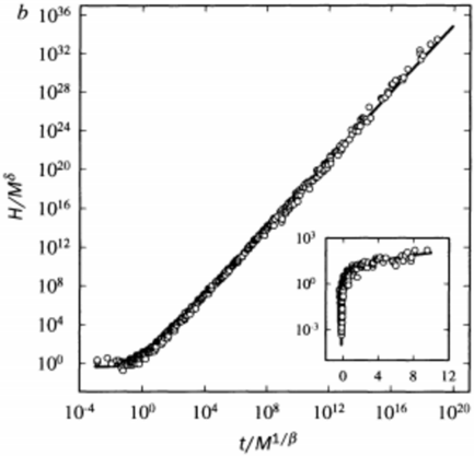
## Line Chart: Log-Log Plot of b vs. t/M^(1/β) ### Overview The image displays a log-log line chart with two axes: the y-axis labeled "b" (ranging from 10⁰ to 10¹⁶) and the x-axis labeled "t/M^(1/β)" (ranging from 10⁻⁴ to 10²⁰). A primary data series is plotted as black circular markers, forming a straight line on the log-log scale. An inset graph in the bottom-right corner zooms into the lower x-axis range (0 to 12) with a y-axis range of 10⁻³ to 10³. The data points in both plots align closely with a straight line, suggesting a power-law relationship. ### Components/Axes - **Y-Axis (Left)**: Labeled "b" with logarithmic scale (10⁰ to 10¹⁶). - **X-Axis (Bottom)**: Labeled "t/M^(1/β)" with logarithmic scale (10⁻⁴ to 10²⁰). - **Inset Graph**: - X-Axis: 0 to 12 (linear scale). - Y-Axis: 10⁻³ to 10³ (logarithmic scale). - **Data Series**: Black circular markers (no explicit legend, but consistent with the main plot). ### Detailed Analysis - **Main Plot**: - Data points form a straight line on the log-log scale, indicating a power-law relationship: $ b \propto \left(\frac{t}{M^{1/\beta}}\right)^k $, where $ k $ is the slope. - The slope appears to be approximately 1 (based on the linear alignment in log-log space). - At $ t/M^{1/\beta} = 10^4 $, $ b \approx 10^8 $; at $ t/M^{1/\beta} = 10^{12} $, $ b \approx 10^{12} $. - **Inset Plot**: - Data points also form a straight line but with a steeper slope (suggesting a higher exponent $ k $ in this regime). - At $ t/M^{1/\beta} = 4 $, $ b \approx 10^0 $; at $ t/M^{1/\beta} = 12 $, $ b \approx 10^3 $. ### Key Observations - The main plot exhibits a consistent power-law trend across the entire x-axis range. - The inset highlights a region where the slope is steeper, possibly indicating a transition or different scaling behavior at lower $ t/M^{1/\beta} $. - No outliers or anomalies are visible in either plot. ### Interpretation The data suggests a universal scaling law where $ b $ depends on $ t/M^{1/\beta} $ via a power-law relationship. The straight-line alignment in the log-log plot confirms this, with the slope $ k $ quantifying the exponent. The inset may represent a specific regime (e.g., early-time behavior or a critical threshold) where the scaling exponent differs, though the exact physical or mathematical context is not provided. The absence of a legend or explicit units for "b" and "t/M^(1/β)" limits direct interpretation, but the log-log scaling implies a dimensionless or normalized quantity. This could relate to phenomena in physics, engineering, or complex systems where self-similarity or scaling invariance is observed.