## Scatter Plot with Linear Fits: Gradient Updates vs. Dimension
### Overview
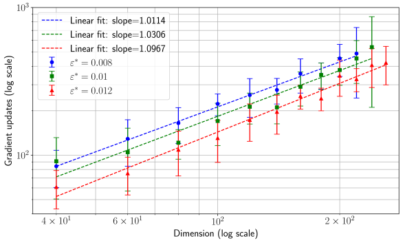
This is a log-log scatter plot with error bars and overlaid linear regression lines. It visualizes the relationship between the dimensionality of a problem (x-axis) and the number of gradient updates required (y-axis) for three different error tolerance levels (ε*). The plot demonstrates a power-law scaling relationship.
### Components/Axes
* **X-Axis:** "Dimension (log scale)". Major tick marks are at `4 × 10¹` (40), `6 × 10¹` (60), `10²` (100), and `2 × 10²` (200). The scale is logarithmic.
* **Y-Axis:** "Gradient updates (log scale)". Major tick marks are at `10²` (100) and `10³` (1000). The scale is logarithmic.
* **Legend (Top-Left Corner):**
* **Linear Fits (Dashed Lines):**
* Blue dashed line: "Linear fit: slope=1.0114"
* Green dashed line: "Linear fit: slope=1.0306"
* Red dashed line: "Linear fit: slope=1.0967"
* **Data Series (Points with Error Bars):**
* Blue circle with error bars: `ε* = 0.008`
* Green circle with error bars: `ε* = 0.01`
* Red circle with error bars: `ε* = 0.012`
* **Grid:** A light gray grid is present for both major and minor ticks on both axes.
### Detailed Analysis
The plot contains three data series, each with 5 data points corresponding to approximate dimensions of 40, 60, 100, 150, and 200. All series show a positive, near-linear trend on this log-log scale.
**Trend Verification & Data Points (Approximate):**
1. **Blue Series (ε* = 0.008):** The line slopes upward consistently. Points (Dimension, Gradient Updates):
* (40, ~80)
* (60, ~120)
* (100, ~200)
* (150, ~300)
* (200, ~400)
* *Associated Linear Fit Slope: 1.0114*
2. **Green Series (ε* = 0.01):** The line slopes upward, positioned slightly below the blue series. Points (Dimension, Gradient Updates):
* (40, ~70)
* (60, ~100)
* (100, ~170)
* (150, ~250)
* (200, ~350)
* *Associated Linear Fit Slope: 1.0306*
3. **Red Series (ε* = 0.012):** The line slopes upward, positioned the lowest of the three. Points (Dimension, Gradient Updates):
* (40, ~50)
* (60, ~80)
* (100, ~130)
* (150, ~200)
* (200, ~280)
* *Associated Linear Fit Slope: 1.0967*
**Error Bars:** All data points have vertical error bars indicating variability. The size of the error bars generally increases with dimension for all series, with the largest bars appearing at dimension 200.
### Key Observations
1. **Consistent Hierarchy:** For any given dimension, a smaller error tolerance (ε*) requires more gradient updates. The order is consistently Blue (ε*=0.008) > Green (ε*=0.01) > Red (ε*=0.012).
2. **Power-Law Scaling:** The linear fits on the log-log plot indicate a relationship of the form: `Gradient Updates ∝ (Dimension)^slope`. All slopes are slightly greater than 1 (ranging from ~1.01 to ~1.10).
3. **Slope vs. Tolerance:** The slope of the linear fit increases as the error tolerance (ε*) increases. The red series (highest ε*) has the steepest slope (1.0967).
4. **Increasing Variance:** The uncertainty (error bar size) in the number of gradient updates grows as the problem dimension increases.
### Interpretation
This plot likely comes from an analysis of optimization algorithms (e.g., in machine learning or numerical analysis). It demonstrates how the computational cost (measured in gradient updates) scales with the problem's dimensionality for different target accuracy levels.
* **Core Finding:** The number of gradient updates scales nearly linearly with dimension (slope ≈ 1), but with a slight super-linear component. This is a favorable scaling property, suggesting the algorithm is relatively efficient in high dimensions.
* **Trade-off:** There is a clear trade-off between solution accuracy and computational cost. Demanding a smaller error (lower ε*) shifts the entire cost curve upward.
* **Increasing Slope with Tolerance:** The observation that the slope increases with ε* is subtle but important. It suggests that for looser error tolerances (higher ε*), the cost grows *slightly faster* with dimension than for tighter tolerances. This could imply that achieving coarse solutions becomes disproportionately more expensive in very high dimensions compared to achieving precise solutions, though the effect is small.
* **Practical Implication:** When scaling a problem to higher dimensions, one must budget for a near-linear increase in computational effort. The large error bars at high dimensions also indicate that performance becomes less predictable as dimensionality grows.