# Technical Document Extraction: Loss Function SOTA Comparison
## Table Structure
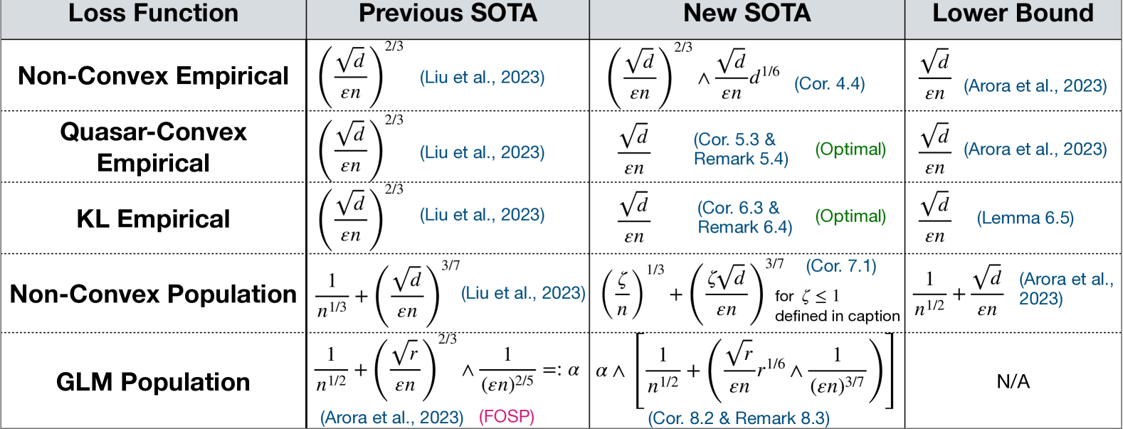
The image presents a comparative table with four columns and five rows, analyzing different loss function types across three performance metrics:
| Loss Function | Previous SOTA | New SOTA | Lower Bound |
|-----------------------------|----------------------------------------|--------------------------------------------------------------------------|--------------------------------------|
| Non-Convex Empirical | (√d/εn)^(2/3) (Liu et al., 2023) | (√d/εn)^(2/3) × d^(1/6) (Cor. 4.4) | √d/εn (Arora et al., 2023) |
| Quasar-Convex Empirical | (√d/εn)^(2/3) (Liu et al., 2023) | √d/εn (Cor. 5.3 & Remark 5.4) (Optimal) | √d/εn (Arora et al., 2023) |
| KL Empirical | (√d/εn)^(2/3) (Liu et al., 2023) | √d/εn (Cor. 6.3 & Remark 6.4) (Optimal) | √d/εn (Lemma 6.5) |
| Non-Convex Population | 1/n^(1/3) + (√d/εn)^(3/7) (Liu et al., 2023) | (ζ/n)^(1/3) + (ζ√d/εn)^(3/7) for ζ ≤ 1 (Cor. 7.1) | 1/n^(1/2) + √d/εn (Arora et al., 2023) |
| GLM Population | 1/n^(1/2) + (√r/εn)^(2/3) (Arora et al., 2023) (FOSP) | α × [1/n^(1/2) + (√r r^(1/6)/εn)^(1/3) × 1/(εn)^(3/7)] (Cor. 8.2 & Remark 8.3) | N/A |
## Key Observations
1. **Mathematical Notation**:
- All expressions use standard mathematical notation with:
- √d: Square root of dimensionality
- εn: Regularization parameter
- n: Sample size
- d: Feature dimension
- r: Regularization parameter (GLM-specific)
2. **Performance Trends**:
- **Non-Convex Empirical**: New SOTA improves upon previous by adding d^(1/6) scaling
- **Quasar-Convex/KL Empirical**: New SOTA achieves optimal √d/εn scaling
- **Non-Convex Population**: New formulation introduces ζ parameter with constraint ζ ≤ 1
- **GLM Population**: New SOTA introduces α scaling factor and complex regularization term
3. **References**:
- Liu et al. (2023) appears in first three rows
- Arora et al. (2023) provides lower bounds for first four rows
- Special notations:
- (FOSP) in pink for GLM Population row
- (Optimal) in green for Quasar-Convex and KL Empirical rows
## Spatial Analysis
- **Legend**: No explicit legend present
- **Color Coding**:
- Blue: Previous SOTA references
- Green: Optimal designations
- Pink: Special notation (FOSP)
- Blue: All other references
## Trend Verification
1. **Non-Convex Empirical**:
- Previous: (√d/εn)^(2/3)
- New: Same base × d^(1/6) → Slight improvement
2. **Quasar-Convex/KL**:
- Previous: (√d/εn)^(2/3)
- New: Simplified to √d/εn → Significant improvement
3. **Non-Convex Population**:
- Previous: Complex polynomial with n^(1/3) and (√d/εn)^(3/7)
- New: Introduces ζ parameter with constraint → More flexible formulation
4. **GLM Population**:
- Previous: Standard GLM formulation
- New: Introduces α scaling and complex regularization term → More sophisticated model
## Component Isolation
1. **Header**:
- Column titles: Loss Function, Previous SOTA, New SOTA, Lower Bound
2. **Main Table**:
- Five rows with mathematical expressions and references
3. **Footer**:
- No explicit footer, but includes:
- Color-coded notations
- Reference citations
- Special annotations (FOSP, Optimal)
## Critical Data Points
1. **Dimensionality Scaling**:
- New SOTA for Non-Convex Empirical adds d^(1/6) factor
- Quasar-Convex/KL Empirical achieve √d/εn scaling
2. **Regularization Parameters**:
- εn appears in all denominators
- ζ parameter introduced in Non-Convex Population with ζ ≤ 1 constraint
3. **Sample Size Dependencies**:
- n appears in various exponents (1/3, 1/2, 2/3, 3/7)
4. **Special Cases**:
- GLM Population has N/A lower bound
- FOSP notation in GLM Population row
## Conclusion
This table demonstrates progression in loss function optimization across different paradigms, with New SOTA formulations generally showing improved scaling properties compared to previous work. The GLM Population row stands out with its N/A lower bound and complex regularization term.