## Diagram & Chart: Approximate Message Passing (AMP) Algorithm & Reconstruction Performance
### Overview
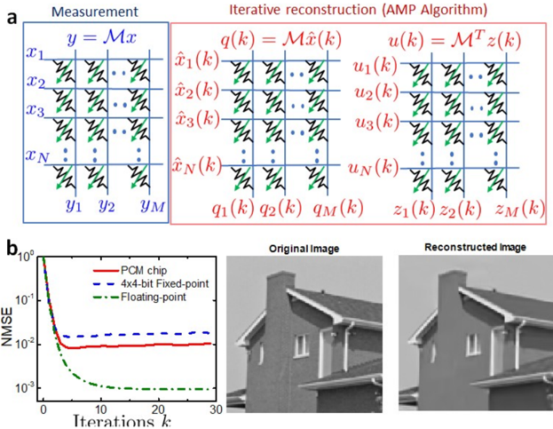
The image presents a visual explanation of the Approximate Message Passing (AMP) algorithm for iterative reconstruction, alongside a performance comparison of different numerical precisions. The top portion (a) illustrates the AMP algorithm's flow with matrix operations and vector updates. The bottom portion (b) shows a chart comparing the Normalized Mean Squared Error (NMSE) for different precision levels (PCM chip, 4x4-bit Fixed-point, and Floating-point) as a function of iterations, and visual examples of original and reconstructed images.
### Components/Axes
**Part a (AMP Algorithm Diagram):**
* **Header:** "Measurement" and "Iterative reconstruction (AMP Algorithm)"
* **Variables:** `y`, `x1` to `xN`, `q1` to `qM`, `u1` to `uN`, `z1` to `zM`
* **Matrices:** `M`, `M̂`, `MT`
* **Equation:** `y = Mx`
* **Equation:** `q(k) = M̂(k)`
* **Equation:** `u(k) = MT z(k)`
**Part b (Performance Chart):**
* **X-axis:** "Iterations k" (Scale: 0 to 30)
* **Y-axis:** "NMSE" (Scale: 10^-2 to 10^0, logarithmic)
* **Legend:**
* Red Solid Line: "PCM chip"
* Red Dashed Line: "4x4-bit Fixed-point"
* Green Dashed Line: "Floating-point"
* **Images:** "Original Image" and "Reconstructed Image" (side-by-side comparison)
### Detailed Analysis or Content Details
**Part a (AMP Algorithm Diagram):**
The diagram shows a series of matrix-vector operations.
* The "Measurement" section shows a matrix `M` multiplying a vector `x` (with components `x1` to `xN`) to produce a vector `y` (with components `y1` to `yM`). The elements of `M` are represented by small green arrows.
* The "Iterative reconstruction" section shows three stages:
1. `q(k) = M̂(k)`: An estimated matrix `M̂` (with elements represented by green arrows) is used to calculate `q(k)` (with components `q1` to `qM`).
2. `u(k) = MT z(k)`: The transpose of `M` (`MT`) is multiplied by `z(k)` (with components `z1` to `zM`) to produce `u(k)` (with components `u1` to `uN`).
3. The diagram shows iterative updates with `x̂1(k)` to `x̂N(k)` and the corresponding `q` and `z` vectors at each iteration `k`.
**Part b (Performance Chart):**
* **Floating-point:** The green dashed line representing Floating-point precision shows a steep downward trend initially, rapidly decreasing from approximately 10^0 to approximately 10^-3 NMSE within the first 10 iterations. The line then plateaus, with minimal further reduction in NMSE. At iteration 30, the NMSE is approximately 2x10^-3.
* **4x4-bit Fixed-point:** The red dashed line representing 4x4-bit Fixed-point precision shows a similar initial downward trend, but less steep than Floating-point. It starts at approximately 10^0 and decreases to approximately 5x10^-2 at iteration 30.
* **PCM chip:** The red solid line representing PCM chip precision shows a more gradual decrease in NMSE. It starts at approximately 10^0 and decreases to approximately 8x10^-2 at iteration 30. The line exhibits some oscillations.
* **Images:** The "Original Image" shows a building with visible details. The "Reconstructed Image" appears slightly blurred compared to the original, but retains the overall structure of the building.
### Key Observations
* Floating-point precision achieves the lowest NMSE and fastest convergence.
* 4x4-bit Fixed-point precision performs better than PCM chip precision, but significantly worse than Floating-point.
* The reconstructed image, while not perfect, demonstrates that the AMP algorithm can effectively reconstruct the original image.
* The NMSE curves suggest diminishing returns with increasing iterations beyond a certain point, particularly for Floating-point precision.
### Interpretation
The data demonstrates the impact of numerical precision on the performance of the AMP algorithm for image reconstruction. Floating-point precision provides the highest accuracy and fastest convergence, likely due to its ability to represent a wider range of values with greater precision. Fixed-point and PCM chip precisions introduce quantization errors that limit the algorithm's performance. The visual comparison of the original and reconstructed images confirms the quantitative results, showing that lower precision leads to a slightly degraded reconstruction quality. The logarithmic scale of the NMSE highlights the significant difference in performance between the different precision levels. The AMP algorithm appears to be effective in reconstructing images, but its performance is sensitive to the numerical precision used in the calculations. The plateauing of the NMSE curves suggests that there is a limit to the achievable reconstruction accuracy, even with high-precision arithmetic. This could be due to factors such as noise in the measurements or imperfections in the model used for reconstruction.