## Diagram & Chart: Measurement and Iterative Reconstruction (AMP Algorithm) with Performance Comparison
### Overview
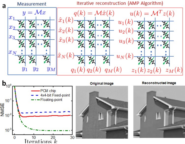
The image is a two-part technical figure illustrating a signal measurement and reconstruction process, alongside a performance comparison of different computational methods. Part (a) is a schematic diagram of the mathematical process. Part (b) contains a line chart comparing reconstruction error over iterations and visual examples of the original and reconstructed images.
### Components/Axes
**Part (a) - Schematic Diagram:**
* **Left Section (Blue Box):** Titled "Measurement". Contains the equation `y = Mx`. It depicts a matrix multiplication where an input vector `x` (with elements `x₁` to `x_N`) is multiplied by a measurement matrix `M` to produce an output vector `y` (with elements `y₁` to `y_M`). The matrix `M` is shown with a pattern of green and black diagonal lines.
* **Right Section (Red Box):** Titled "Iterative reconstruction (AMP Algorithm)". It shows two key equations:
1. `q(k) = Mx̂(k)`: This operation takes the current estimate `x̂(k)` (with elements `x̂₁(k)` to `x̂_N(k)`) and multiplies it by the same measurement matrix `M` to produce `q(k)` (with elements `q₁(k)` to `q_M(k)`).
2. `u(k) = Mᵀz(k)`: This operation takes a vector `z(k)` (with elements `z₁(k)` to `z_M(k)`) and multiplies it by the transpose of the measurement matrix `Mᵀ` to produce `u(k)` (with elements `u₁(k)` to `u_N(k)`).
* **Spatial Grounding:** The "Measurement" box is on the left. The "Iterative reconstruction" box is on the right, containing the two sub-processes side-by-side. The matrix `M` in both sections has an identical visual pattern.
**Part (b) - Line Chart & Images:**
* **Chart Title:** None explicitly stated. The Y-axis is labeled "NMSE" (Normalized Mean Square Error). The X-axis is labeled "Iterations k".
* **Y-Axis:** Logarithmic scale ranging from `10⁻³` to `10⁰`.
* **X-Axis:** Linear scale from 0 to 30.
* **Legend (Top-Left of chart):**
* `PCM chip` (Red, solid line)
* `4x4-bit Fixed-point` (Blue, dashed line)
* `Floating-point` (Green, dash-dot line)
* **Images (Right of chart):** Two grayscale images placed side-by-side.
* Left image label: "Original Image"
* Right image label: "Reconstructed Image"
* Both show the same architectural subject: a house with a prominent chimney, rooflines, and windows.
### Detailed Analysis
**Chart Data Trends & Approximate Values:**
1. **PCM chip (Red, solid):** Starts at NMSE ≈ `10⁰` (1.0) at k=0. Drops sharply to ≈ `2 x 10⁻²` by k=5. From k=5 to k=30, it remains relatively stable, plateauing around `1-2 x 10⁻²`.
2. **4x4-bit Fixed-point (Blue, dashed):** Starts at NMSE ≈ `10⁰`. Drops to ≈ `3 x 10⁻²` by k=5. It then plateaus at a slightly higher error level than the PCM chip line, approximately `2-3 x 10⁻²` from k=5 to k=30.
3. **Floating-point (Green, dash-dot):** Starts at NMSE ≈ `10⁰`. Shows the steepest and most sustained descent. Crosses below the other two lines before k=5. Continues to decrease, reaching ≈ `10⁻³` by k=15 and approaching `~8 x 10⁻⁴` by k=30.
**Visual Image Comparison:**
The "Reconstructed Image" appears visually very similar to the "Original Image". Key structural features (chimney, roof edges, windows) are preserved. There may be a slight loss of fine texture or subtle blurring in the reconstructed version, but no major artifacts or distortions are immediately apparent at this scale.
### Key Observations
1. **Convergence Behavior:** All three methods show rapid error reduction in the first 5 iterations, after which the error plateaus. The floating-point method is the only one that continues to show meaningful improvement beyond 10 iterations.
2. **Performance Hierarchy:** The floating-point method achieves the lowest final NMSE (best reconstruction quality). The PCM chip method performs slightly better than the 4x4-bit fixed-point method, which has the highest plateaued error.
3. **Visual Fidelity:** Despite the numerical differences in NMSE, the final reconstructed image for the method shown (presumably the PCM chip, given its prominence) is of high visual quality, closely matching the original.
### Interpretation
This figure demonstrates the application of the Approximate Message Passing (AMP) algorithm for reconstructing a signal (an image) from compressed measurements (`y = Mx`). The diagram in (a) breaks down the core iterative steps of the algorithm.
The chart in (b) provides a quantitative comparison of how different hardware/precision implementations of this algorithm affect reconstruction accuracy over time. The key insight is a **trade-off between computational precision and reconstruction error**:
* **Floating-point** arithmetic offers the highest accuracy (lowest NMSE) but is typically more computationally expensive and power-hungry.
* The **PCM chip** (likely a specialized analog/mixed-signal hardware implementation) and **4x4-bit Fixed-point** (a low-precision digital implementation) converge to a higher, but stable, error floor. This suggests they are efficient, hardware-friendly approximations that sacrifice some accuracy for potential gains in speed, power efficiency, or area.
The fact that the visual quality remains high despite the NMSE plateau indicates that the error may be concentrated in perceptually less significant image components. The figure argues that specialized, lower-precision hardware like the PCM chip can achieve visually satisfactory reconstruction results efficiently, making it a viable option for edge computing or power-constrained applications where floating-point precision is not feasible.