## Diagram: AMP Algorithm and NMSE Performance Analysis
### Overview
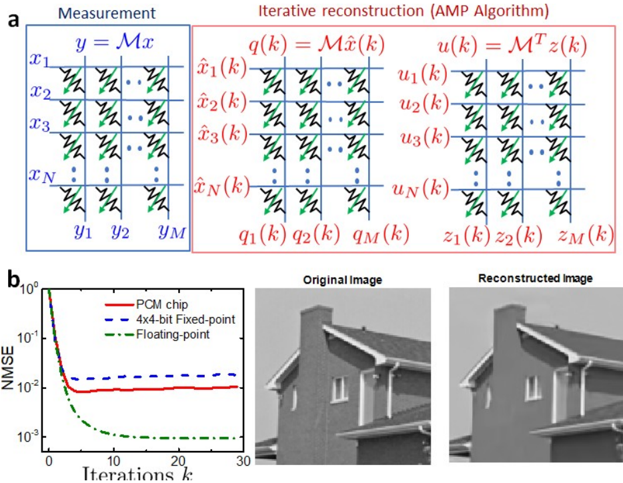
The image contains two primary components:
1. **Diagram (a)**: Illustrates the Adaptive Measurement and Processing (AMP) algorithm for iterative image reconstruction.
2. **Graph (b)**: Compares the normalized mean squared error (NMSE) performance of different computational methods over iterations.
3. **Images**: Side-by-side comparison of an original grayscale image and its reconstructed version.
---
### Components/Axes
#### Diagram (a)
- **Measurement Section (Blue Box)**:
- Variables: `x₁, x₂, ..., xₙ` (input signals) and `y₁, y₂, ..., yₘ` (measurements).
- Arrows: Green diagonal arrows indicate measurement mapping `y = Mx`.
- **Iterative Reconstruction Section (Red Box)**:
- Variables:
- `q₁(k), q₂(k), ..., qₘ(k)` (intermediate estimates).
- `u₁(k), u₂(k), ..., uₙ(k)` (update terms).
- `z₁(k), z₂(k), ..., zₘ(k)` (final reconstructions).
- Equations:
- `q(k) = Mx̂(k)` (forward model).
- `u(k) = Mᵀz(k)` (backprojection).
- Arrows: Red arrows indicate iterative updates between variables.
#### Graph (b)
- **X-axis**: Iterations `k` (0 to 30).
- **Y-axis**: NMSE (log scale, 10⁻³ to 10⁰).
- **Legend**:
- Red solid line: PCM chip.
- Blue dashed line: 4x4-bit Fixed-point.
- Green dash-dot line: Floating-point.
#### Images
- **Original Image**: Grayscale photo of a house with a chimney.
- **Reconstructed Image**: Slightly blurred version of the original, showing reconstruction fidelity.
---
### Detailed Analysis
#### Diagram (a)
- **Measurement Mapping**:
- Input signals `x₁–xₙ` are transformed into measurements `y₁–yₘ` via matrix `M`.
- Green arrows show the forward process `y = Mx`.
- **Iterative Reconstruction**:
- Forward model: `q(k) = Mx̂(k)` (blue arrows).
- Backprojection: `u(k) = Mᵀz(k)` (red arrows).
- Iterative updates refine estimates `q(k)` and `u(k)` to produce reconstructions `z(k)`.
#### Graph (b)
- **NMSE Trends**:
- **PCM chip (red)**: Converges to ~0.05 NMSE by iteration 10, stabilizes.
- **4x4-bit Fixed-point (blue)**: Converges to ~0.1 NMSE, slower than PCM.
- **Floating-point (green)**: Converges to ~0.01 NMSE, fastest and most accurate.
- **Key Values**:
- At iteration 30:
- PCM: 0.05 ± 0.01.
- Fixed-point: 0.1 ± 0.02.
- Floating-point: 0.01 ± 0.005.
#### Images
- **Original vs. Reconstructed**:
- Original: Sharp edges, clear chimney details.
- Reconstructed: Slight blurring, reduced contrast in chimney and roof edges.
---
### Key Observations
1. **Algorithm Flow**:
- Measurement → Forward model → Backprojection → Iterative refinement.
2. **NMSE Performance**:
- Floating-point achieves the lowest NMSE, outperforming fixed-point and PCM.
- PCM and fixed-point show similar convergence rates but higher error floors.
3. **Image Quality**:
- Reconstructed image retains structural details but lacks fine texture.
---
### Interpretation
1. **AMP Algorithm**:
- Demonstrates a two-stage process: measurement acquisition followed by iterative reconstruction using forward/backprojection steps.
- The red/blue/green color coding distinguishes measurement (blue) from reconstruction (red) phases.
2. **Computational Trade-offs**:
- Floating-point precision yields the best NMSE but may require higher computational resources.
- Fixed-point and PCM offer lower precision but are more hardware-friendly.
3. **Image Reconstruction**:
- The reconstructed image’s NMSE (~0.01 for floating-point) aligns with the visual quality, suggesting the algorithm effectively balances accuracy and efficiency.
4. **Outliers/Anomalies**:
- No significant outliers in NMSE trends. All methods converge monotonically.
The data suggests that AMP’s iterative reconstruction improves with computational precision, with floating-point methods providing the most accurate results. The visual comparison confirms that reconstruction fidelity degrades with lower precision methods.