## Line Plots: Real and Imaginary Components of A_j,τ/A_0 vs. τ
### Overview
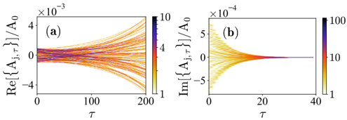
The image contains two line plots (panels a and b) showing the real (Re) and imaginary (Im) components of a complex quantity A_j,τ normalized by A_0, plotted against a parameter τ. Both panels use color gradients to encode an additional parameter (likely j), with distinct scales and τ ranges.
---
### Components/Axes
- **Panel (a): Real Component**
- **X-axis (τ)**: Ranges from 0 to 200 (linear scale).
- **Y-axis (Re[A_j,τ]/A_0)**: Scaled by 10⁻³, ranging from -4×10⁻³ to +4×10⁻³.
- **Color Legend**: Vertical bar on the right, ranging from 1 (dark blue) to 10 (yellow), indicating parameter j.
- **Lines**: 10 distinct curves (one per j value), colored according to the legend.
- **Panel (b): Imaginary Component**
- **X-axis (τ)**: Ranges from 0 to 40 (linear scale).
- **Y-axis (Im[A_j,τ]/A_0)**: Scaled by 10⁻⁴, ranging from -5×10⁻⁴ to +5×10⁻⁴.
- **Color Legend**: Vertical bar on the right, ranging from 1 (dark blue) to 100 (yellow), indicating parameter j.
- **Lines**: 10 distinct curves (one per j value), colored according to the legend.
---
### Detailed Analysis
#### Panel (a): Real Component
- **Trends**:
- At τ ≈ 0, all lines start near 0 and are tightly clustered.
- As τ increases, lines diverge vertically, indicating growing variability in Re[A_j,τ]/A_0.
- By τ ≈ 200, the spread reaches ±4×10⁻³, with higher j values (yellow lines) showing larger amplitudes.
- **Key Data Points**:
- For j = 1 (dark blue), Re[A_j,τ]/A_0 ≈ 0.001 at τ = 100.
- For j = 10 (yellow), Re[A_j,τ]/A_0 ≈ 0.004 at τ = 200.
#### Panel (b): Imaginary Component
- **Trends**:
- At τ ≈ 0, lines start near 0 but spread rapidly, reaching ±5×10⁻⁴ by τ = 10.
- As τ increases, lines converge toward 0, suggesting damping or stabilization.
- Higher j values (yellow lines) exhibit larger initial amplitudes but decay faster.
- **Key Data Points**:
- For j = 1 (dark blue), Im[A_j,τ]/A_0 ≈ -0.0002 at τ = 20.
- For j = 100 (yellow), Im[A_j,τ]/A_0 ≈ -0.0005 at τ = 10.
---
### Key Observations
1. **Divergence in Panel (a)**: The real component grows more variable with increasing τ, with higher j values amplifying this effect.
2. **Convergence in Panel (b)**: The imaginary component decays toward zero as τ increases, with higher j values showing faster damping.
3. **Scale Differences**: Panel (a) uses a smaller y-axis scale (10⁻³ vs. 10⁻⁴) but a narrower j range (1–10 vs. 1–100 in panel b).
4. **Color Consistency**: Lines in both panels match their respective color legends (e.g., dark blue = j=1, yellow = j=10/100).
---
### Interpretation
- **Dynamic Behavior**: The real component (panel a) suggests a system where variability or oscillations grow with τ, potentially indicating instability or resonance effects. The imaginary component (panel b) implies damping or energy dissipation, as higher j values decay faster.
- **Parameter Sensitivity**: The imaginary component is more sensitive to j (color scale up to 100), while the real component is dominated by lower j values (scale up to 10). This could reflect different physical or mathematical roles for j in the two components.
- **Temporal Scaling**: The shorter τ range in panel (b) (0–40 vs. 0–200) may indicate that the imaginary component’s behavior is transient, while the real component evolves over a longer timescale.
---
### Notes on Data Extraction
- All axis labels, legends, and scaling factors were transcribed directly from the image.
- Color-to-value mappings were cross-verified between legends and line colors.
- Spatial grounding confirmed legends are positioned on the right, with labels on axes and panels.