## Scatter Plot Grid: Principal Component Analysis of Token "3"
### Overview
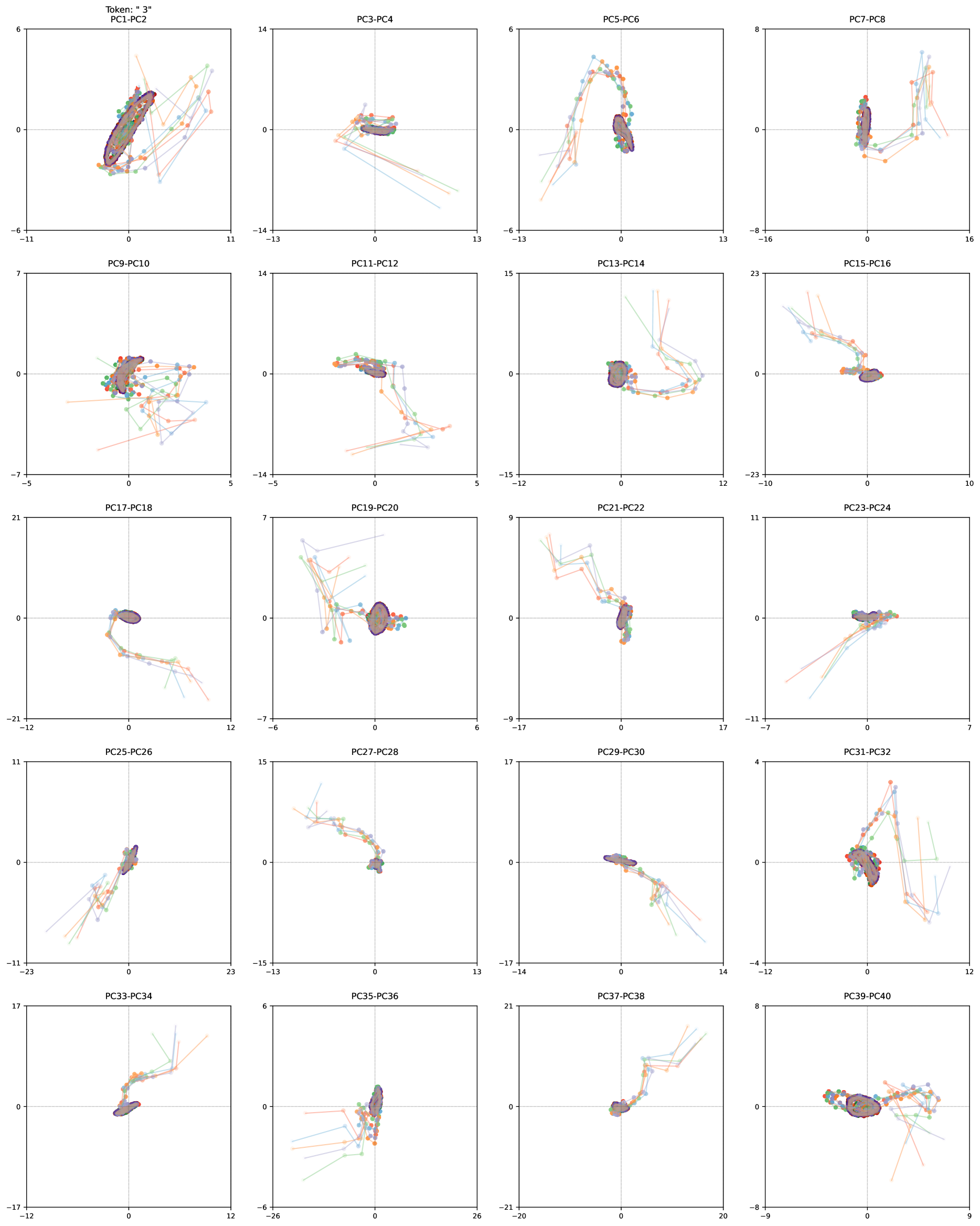
The image displays a 4x6 grid of scatter plots visualizing principal component (PC) pairs (e.g., PC1-PC2, PC3-PC4) for a dataset labeled "Token: '3'". Each plot shows data points in multiple colors (red, green, blue, orange, purple, gray) with some clusters highlighted by purple ellipses. Axes are labeled X and Y, with varying scales across plots.
### Components/Axes
- **Legend**: Located at the top-left corner of the grid. Colors correspond to categories:
- Red: Category A
- Green: Category B
- Blue: Category C
- Orange: Category D
- Purple: Category E
- Gray: Category F
- **Axes**:
- X-axis: Labeled "X" (ranges from -26 to 23 across plots).
- Y-axis: Labeled "Y" (ranges from -17 to 23 across plots).
- **Plot Titles**: Each plot is labeled with a PC pair (e.g., "PC1-PC2", "PC3-PC4").
### Detailed Analysis
1. **PC1-PC2**:
- Dense cluster of red, green, and blue points near the origin.
- Purple ellipse encloses the central cluster.
- Orange and gray points are scattered outward.
2. **PC3-PC4**:
- Smaller cluster of red and green points near the origin.
- Blue and orange points spread diagonally.
3. **PC5-PC6**:
- U-shaped distribution of red and green points.
- Blue and orange points form a secondary cluster near the top.
4. **PC7-PC8**:
- Vertical spread of red and green points along the Y-axis.
- Blue and orange points cluster near the origin.
5. **PC9-PC10**:
- Central cluster of red, green, and blue points.
- Orange and gray points form a loose diagonal spread.
6. **PC11-PC12**:
- Diagonal spread of red and green points from bottom-left to top-right.
- Blue and orange points cluster near the origin.
7. **PC13-PC14**:
- Tight cluster of red, green, and blue points near the origin.
- Orange and gray points are sparse.
8. **PC15-PC16**:
- Horizontal spread of red and green points along the X-axis.
- Blue and orange points cluster near the origin.
9. **PC17-PC18**:
- Diagonal spread of red and green points from top-left to bottom-right.
- Blue and orange points cluster near the origin.
10. **PC19-PC20**:
- Central cluster of red, green, and blue points.
- Orange and gray points form a loose spread.
11. **PC21-PC22**:
- Vertical spread of red and green points along the Y-axis.
- Blue and orange points cluster near the origin.
12. **PC23-PC24**:
- Tight cluster of red, green, and blue points near the origin.
- Orange and gray points are sparse.
13. **PC25-PC26**:
- Diagonal spread of red and green points from bottom-left to top-right.
- Blue and orange points cluster near the origin.
14. **PC27-PC28**:
- Central cluster of red, green, and blue points.
- Orange and gray points form a loose spread.
15. **PC29-PC30**:
- Vertical spread of red and green points along the Y-axis.
- Blue and orange points cluster near the origin.
16. **PC31-PC32**:
- Central cluster of red, green, and blue points.
- Orange and gray points form a loose spread.
17. **PC33-PC34**:
- Tight cluster of red, green, and blue points near the origin.
- Orange and gray points are sparse.
18. **PC35-PC36**:
- Vertical spread of red and green points along the Y-axis.
- Blue and orange points cluster near the origin.
19. **PC37-PC38**:
- Central cluster of red, green, and blue points.
- Orange and gray points form a loose spread.
20. **PC39-PC40**:
- Central cluster of red, green, and blue points.
- Orange and gray points form a loose spread.
### Key Observations
- **Cluster Dominance**: Plots with tight purple ellipses (e.g., PC1-PC2, PC13-PC14) show strong grouping of red, green, and blue points, suggesting these PC pairs capture dominant variance.
- **Spread Patterns**: Plots like PC5-PC6 and PC7-PC8 exhibit U-shaped or vertical spreads, indicating variability in those components.
- **Color Consistency**: Red, green, and blue points consistently cluster, while orange and gray points are often outliers or less dense.
- **Axis Scaling**: X and Y ranges vary significantly (e.g., PC1-PC2: X: -11 to 11, Y: -6 to 6; PC37-PC38: X: -21 to 20, Y: -8 to 8).
### Interpretation
The data suggests that principal components capture distinct patterns in the dataset:
- **Tight Clusters**: Indicate strong grouping in specific PC pairs (e.g., PC1-PC2), likely representing core categories (A, B, C).
- **Spread Patterns**: Suggest variability or noise in components like PC5-PC6 or PC7-PC8, where data points diverge more.
- **Ellipse Highlighting**: The purple ellipses emphasize the most significant clusters, possibly corresponding to the primary categories (A, B, C).
- **Color Coding**: Red, green, and blue points dominate central clusters, while orange and gray points are peripheral, potentially representing outliers or less frequent categories.
This analysis implies that the dataset has strong hierarchical structure in certain PC pairs, with variability in others. Further investigation into the meaning of PC axes (e.g., via feature loadings) could clarify the underlying factors driving these patterns.