## Line Chart: Learning Rate ### Overview The image is a line chart displaying the learning rate over the course of training, measured in samples. The learning rate initially increases rapidly, plateaus, and then decreases in two stages. ### Components/Axes * **Title:** Learning Rate * **X-axis:** sample * Scale: 0 to 1.5G (1.5 * 10^9), with tick marks at 500M (5 * 10^8) and 1G (1 * 10^9). * **Y-axis:** Learning Rate * Scale: 0 to 0.0008, with tick marks at 0.0002 intervals. ### Detailed Analysis * **Data Series:** The single data series is represented by a blue line. * **Trend:** The line initially rises sharply, plateaus at approximately 0.0008, then drops to approximately 0.0006, remains constant for a while, and then decreases linearly in two segments. * **Data Points:** * Starts near 0. * Rises sharply to approximately 0.0008 before 500M samples. * Drops to approximately 0.0006 before 500M samples. * Remains at approximately 0.0006 until approximately 1G samples. * Decreases to approximately 0.0004 at approximately 1.5G samples. * Decreases further to approximately 0.00027 after 1.5G samples. ### Key Observations * The learning rate experiences an initial rapid increase. * The learning rate plateaus at two different levels. * The learning rate decreases linearly in two distinct segments towards the end of the training. ### Interpretation The chart illustrates a learning rate schedule commonly used in machine learning. The initial rapid increase allows for quick learning at the beginning of training. The plateau phase maintains a consistent learning rate. The final decrease helps to fine-tune the model and avoid overshooting the optimal parameters. The two-stage decrease suggests a more granular approach to fine-tuning, potentially targeting different aspects of the model.

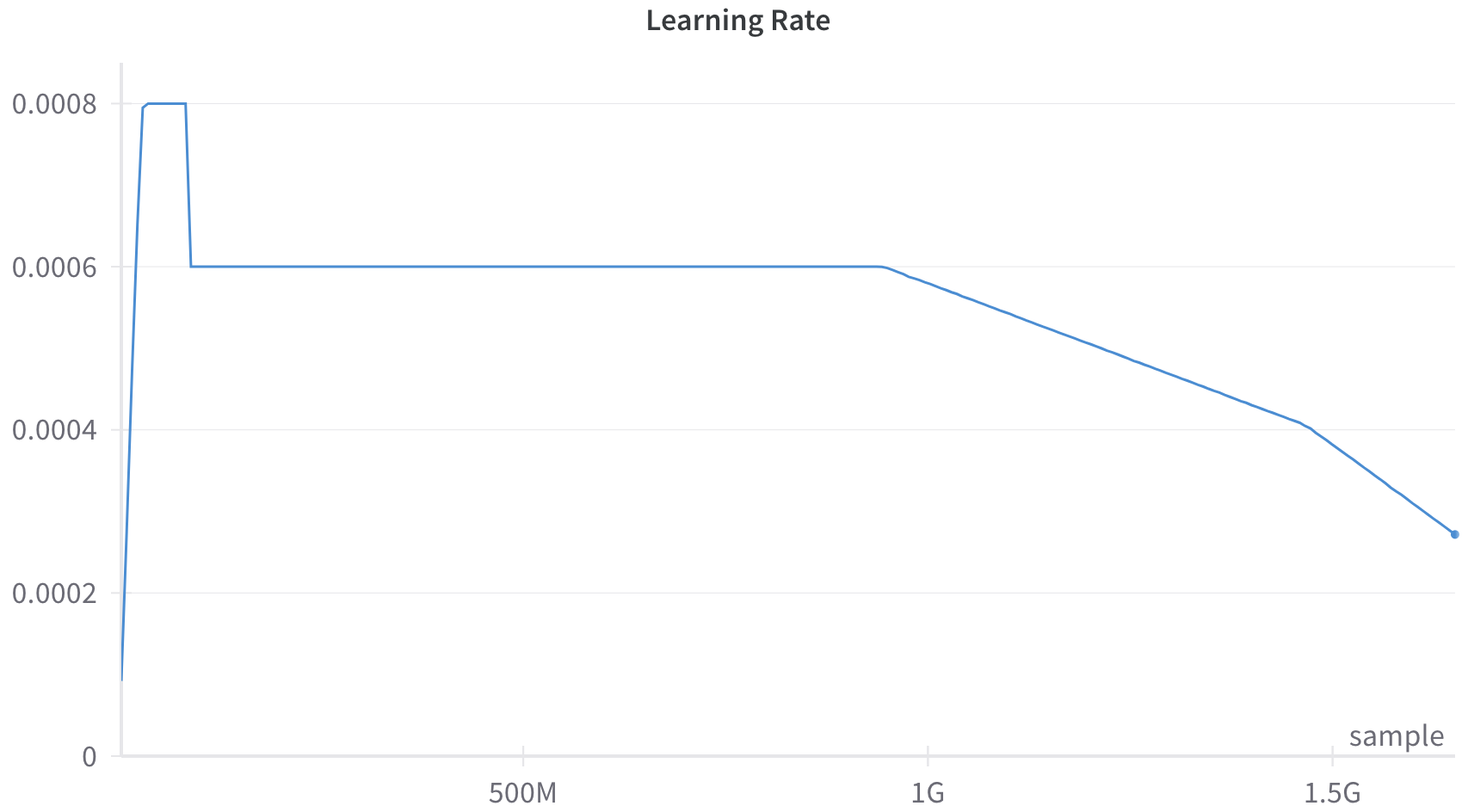
## Line Chart: Learning Rate Schedule ### Overview This image is a line chart displaying a "Learning Rate" schedule over a number of training samples. The chart features a single blue line that illustrates a specific learning rate strategy, characterized by an initial sharp warmup, a brief peak, a step-down to a sustained plateau, and a final linear decay phase. All text in the image is in English. ### Components/Axes **Header Region:** * **Title:** "Learning Rate" (Located top-center, dark gray text). **Main Chart Region:** * **Data Series:** A single solid blue line representing the learning rate value. It ends with a distinct blue circular marker (dot) at the final data point. * **Grid:** Four light gray horizontal grid lines corresponding to the Y-axis major tick marks (excluding 0). There are no vertical grid lines. * **Legend:** There is no legend present, as there is only a single data series. **Axes/Footer Region:** * **Y-axis (Left):** Represents the learning rate value. It has a solid light gray axis line. * **Markers (Bottom to Top):** `0`, `0.0002`, `0.0004`, `0.0006`, `0.0008`. * **Label:** There is no explicit Y-axis label, though the chart title "Learning Rate" serves this purpose. * **X-axis (Bottom):** Represents the number of samples processed. It has a solid light gray axis line with small vertical tick marks. * **Markers (Left to Right):** * [Origin]: Implicitly 0. * `500M` (Located at approximately 30% of the axis width). * `1G` (Located at approximately 60% of the axis width). * `1.5G` (Located at approximately 90% of the axis width). * **Label:** "sample" (Located at the bottom-right, just above the X-axis line). * *Note on scale:* 'M' denotes Millions, and 'G' denotes Billions (Giga). ### Detailed Analysis **Trend Verification and Data Extraction:** The single blue line exhibits four distinct phases. 1. **Warmup Phase (Steep Upward Slope):** * *Trend:* The line starts slightly above zero and slopes upward almost vertically. * *Data Points:* Starts at X = 0, Y ≈ 0.0001. It rises sharply to reach Y = 0.0008 at an estimated X ≈ 50M. 2. **Peak Phase (Flat Horizontal Line):** * *Trend:* The line remains perfectly flat at its maximum value for a brief period. * *Data Points:* Maintains Y = 0.0008 from X ≈ 50M to X ≈ 100M. 3. **Plateau Phase (Step-down and Flat Horizontal Line):** * *Trend:* The line drops vertically, then remains perfectly flat for the majority of the chart. * *Data Points:* At X ≈ 100M, the value drops sharply from Y = 0.0008 to Y = 0.0006. It then holds steady at Y = 0.0006 across the 500M mark, continuing until just before the 1G mark (estimated X ≈ 950M). 4. **Decay Phase (Downward Linear Slope):** * *Trend:* The line slopes downward at a constant, linear rate until the end of the chart. * *Data Points:* The decay begins at X ≈ 950M, Y = 0.0006. It crosses exactly through the grid intersection at X = 1.5G, Y = 0.0004. The line terminates with a distinct dot at an estimated X ≈ 1.75G, with a final Y-value of approximately 0.00027. ### Key Observations * **Anomalous Step-Down:** Unlike standard cosine or linear decay schedules that smoothly transition from a peak, this schedule features a hard, instantaneous step-down from 0.0008 to 0.0006 early in the training process. * **Extended Constant Rate:** The vast majority of the training (from ~100M to ~950M samples) occurs at a static learning rate of 0.0006. * **Linear Decay:** The final phase is strictly linear, rather than curved (exponential or cosine), dropping by exactly 0.0002 over the course of roughly 550M samples (from ~950M to 1.5G). ### Interpretation This chart represents a highly specific, custom learning rate schedule used for training a machine learning model (likely a large neural network, given the scale of billions of samples). * **The Warmup:** The initial spike to 0.0008 is a standard "warmup" phase. This prevents the model's weights from diverging early in training when gradients are large and unstable. * **The Step-Down & Plateau:** The sudden drop to 0.0006 and the long plateau suggest a deliberate design choice. The engineers likely found that 0.0008 was too high for sustained training (perhaps causing instability after the initial warmup), but 0.0006 provided a stable, rapid convergence rate for the bulk of the training process. * **The Linear Decay:** The linear decay starting near 1 Billion samples represents the "fine-tuning" or "annealing" phase. As the model gets closer to an optimal solution, the learning rate is steadily reduced so the model can settle into a local minimum without overshooting it. * **Incomplete Run:** The presence of the dot at the end of the line, combined with the fact that the learning rate has not reached zero, implies that this chart represents a snapshot of a training run that either finished at exactly ~1.75G samples, or was paused/evaluated at that specific point.

\n ## Line Chart: Learning Rate ### Overview The image presents a line chart illustrating the learning rate over a training process, likely measured in terms of the number of samples processed. The chart shows a decreasing learning rate as the training progresses. ### Components/Axes * **Title:** "Learning Rate" - positioned at the top-center of the chart. * **X-axis:** Represents the training progress, labeled with values "0", "500M", "1G", and "1.5G". "M" likely stands for million, and "G" for billion, indicating the number of samples processed. * **Y-axis:** Represents the learning rate, ranging from approximately 0 to 0.008. * **Data Series:** A single blue line representing the learning rate. * **Label:** "sample" - positioned at the bottom-right of the chart. ### Detailed Analysis The blue line representing the learning rate exhibits three distinct phases: 1. **Initial Drop:** The learning rate starts at approximately 0.008 at 0 samples and rapidly decreases to approximately 0.006 at around 100M samples. 2. **Plateau:** The learning rate remains relatively constant at approximately 0.006 between 100M and 1G samples. 3. **Gradual Decline:** From 1G samples onwards, the learning rate gradually decreases from approximately 0.006 to approximately 0.002 at 1.5G samples. Here's a breakdown of approximate data points: * 0 samples: 0.008 * 100M samples: 0.006 * 500M samples: 0.006 * 1G samples: 0.006 * 1.5G samples: 0.002 ### Key Observations The learning rate is initially high to allow for rapid initial learning, then stabilizes for a period, and finally decreases to fine-tune the model and prevent overshooting the optimal solution. The plateau phase suggests a period of stable learning, while the final decline indicates a focus on convergence. ### Interpretation This chart demonstrates a common learning rate scheduling strategy used in machine learning. The initial high learning rate allows the model to quickly move towards a region of low loss. The plateau phase allows for refinement within that region, and the final decay helps to converge to a more precise solution. The "sample" label suggests that the x-axis represents the number of training samples processed. The decreasing learning rate is a technique to improve the stability and performance of the training process, especially as the model approaches a minimum in the loss landscape. The shape of the curve suggests a deliberate strategy to balance exploration (initial high rate) and exploitation (final decay).

## Line Graph: Learning Rate Schedule ### Overview The image displays a line graph titled "Learning Rate," plotting the learning rate value against the number of training samples processed. The graph illustrates a common learning rate schedule used in machine learning model training, featuring distinct phases: a warm-up, a constant period, and a linear decay. ### Components/Axes * **Title:** "Learning Rate" (centered at the top). * **Y-Axis (Vertical):** Represents the learning rate value. It is a linear scale with labeled tick marks at: * 0 * 0.0002 * 0.0004 * 0.0006 * 0.0008 * **X-Axis (Horizontal):** Represents the number of training samples processed. It is labeled "sample" at the bottom-right. The axis has labeled tick marks at: * 500M (500 million) * 1G (1 billion) * 1.5G (1.5 billion) * **Data Series:** A single blue line traces the learning rate value over the sample count. There is no legend, as only one series is present. * **Visual Style:** The graph has a clean, minimal design with a white background. Horizontal grid lines are present only at the labeled y-axis ticks. ### Detailed Analysis The learning rate schedule follows a three-phase pattern: 1. **Warm-up Phase (Approx. 0 to ~50M samples):** The line starts at a value near 0 (approximately 0.0001) and rises very steeply to a peak of **0.0008**. It holds at this peak for a very short, flat segment. 2. **Constant Phase (Approx. ~50M to ~1G samples):** The learning rate drops sharply from 0.0008 to **0.0006**. It then remains perfectly constant at 0.0006 for the majority of the training run, from roughly 50 million samples until just before the 1 billion sample mark. 3. **Decay Phase (Approx. ~1G to 1.5G+ samples):** Beginning at approximately 1 billion samples, the learning rate begins a steady, linear decline. The slope is constant. By the 1.5G sample mark, the learning rate has decreased to approximately **0.0004**. The line continues decaying past this point, ending at a final data point (marked with a small dot) at approximately **0.00027**. **Trend Verification:** The visual trend is clear: a rapid initial increase, a long plateau, and then a consistent downward slope. The extracted numerical values align with this visual progression. ### Key Observations * **Scale of Training:** The x-axis scale (in billions of samples) indicates this schedule is for an extremely large-scale model training run. * **Abrupt Transitions:** The transitions between phases (warm-up to constant, constant to decay) are sharp and immediate, not gradual. * **Final Value:** The learning rate does not decay to zero within the visible graph; it ends at a non-zero value (~0.00027), suggesting training may continue or this is the final scheduled rate. * **Minimalist Design:** The graph contains only the essential elements (axes, labels, line) without additional annotations, markers, or a legend. ### Interpretation This graph depicts a **"warmup + constant + linear decay"** learning rate schedule, a standard technique in training deep neural networks, particularly large language models. * **Purpose of Phases:** * **Warm-up:** The initial rapid increase helps stabilize training early on when model weights are random, preventing large, destabilizing gradient updates. * **Constant Phase:** The long plateau at 0.0006 allows the model to learn steadily and efficiently over the bulk of the training process. * **Linear Decay:** The final decay phase fine-tunes the model. Gradually reducing the learning rate helps the model settle into a good minimum in the loss landscape, improving final performance and generalization. * **Underlying Logic:** The schedule balances exploration (higher learning rates early on) with exploitation (lower learning rates later for precise convergence). The specific values (peak of 0.0008, plateau at 0.0006) and the timing of transitions (at ~1G samples) are critical hyperparameters tuned for this specific model and dataset. * **Scale Context:** The use of "G" (billions) for samples underscores the massive computational scale of modern AI training. This single graph represents a training run that likely required thousands of GPU/TPU hours.

## Line Chart: Learning Rate ### Overview The image depicts a line chart titled "Learning Rate," showing the relationship between the number of samples (x-axis) and the learning rate (y-axis). The chart features a single blue line that exhibits a sharp initial increase, followed by a prolonged flat phase, and a gradual decline toward the end of the sample range. ### Components/Axes - **X-axis (Horizontal)**: Labeled "sample," with values ranging from 0 to 1.5G (1.5 billion). Tick marks are at 0, 500M, 1G, and 1.5G. - **Y-axis (Vertical)**: Labeled "Learning Rate," with values ranging from 0 to 0.0008. Tick marks are at 0.0002, 0.0004, 0.0006, and 0.0008. - **Legend**: Located at the bottom-right corner, labeled "sample" with a blue color. The legend confirms the line's color corresponds to the "sample" data series. - **Line**: A single blue line representing the learning rate over the sample range. ### Detailed Analysis - **Initial Spike**: The line starts near 0.0002 at 0 samples, then sharply rises to 0.0008 within the first 500M samples. This suggests an abrupt increase in the learning rate at the beginning of training. - **Flat Phase**: From 500M to 1G samples, the learning rate remains constant at 0.0008. This indicates a stable phase where the learning rate is not adjusted. - **Gradual Decline**: After 1G samples, the learning rate decreases linearly from 0.0008 to approximately 0.0003 at 1.5G samples. The slope of this decline is consistent, suggesting a controlled reduction in the learning rate. ### Key Observations 1. **Sharp Initial Increase**: The learning rate jumps from ~0.0002 to 0.0008 within the first 500M samples, indicating a possible warm-up phase or aggressive initial training. 2. **Stable Phase**: The flat line from 500M to 1G samples suggests the learning rate was held constant during this period, possibly to allow the model to stabilize. 3. **Gradual Decline**: The linear decrease after 1G samples implies a learning rate scheduler was applied to reduce the rate over time, likely to fine-tune the model and avoid overfitting. ### Interpretation The chart illustrates a learning rate schedule that prioritizes rapid initial training (via the sharp increase) followed by stabilization and gradual refinement. The flat phase (500M–1G samples) may reflect a period where the model's performance was optimized at a fixed learning rate. The subsequent decline could be part of a strategy to reduce the learning rate to improve convergence or prevent overfitting. The absence of error bars or variability in the line suggests the data is presented as a deterministic trend rather than a probabilistic distribution. The use of a single data series (blue line) indicates the chart focuses on a specific training configuration or hyperparameter setting. The x-axis range (up to 1.5G samples) implies the model was trained on a large dataset, with the learning rate adjusted to manage computational efficiency and model performance.