## Combined Line Charts: Eigenvalue Decay and Effective Dimension
### Overview
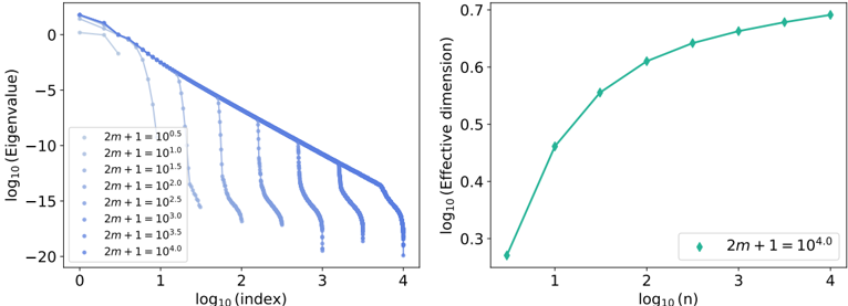
The image presents two line charts side-by-side. The left chart illustrates the decay of eigenvalues as a function of index for different values of the parameter `2m + 1`. The right chart shows the relationship between the effective dimension and `n` for a specific value of `2m + 1`. Both charts use logarithmic scales on their axes.
### Components/Axes
**Left Chart:**
* **Title:** Implicitly, Eigenvalue Decay vs. Index
* **X-axis:** log₁₀(index)
* Scale: 0 to 4
* **Y-axis:** log₁₀(Eigenvalue)
* Scale: -20 to 0
* **Legend:** Located on the left side of the chart. Lists different values for the parameter `2m + 1`:
* `2m + 1 = 10⁰.⁵` (lightest gray)
* `2m + 1 = 10¹.⁰` (light gray)
* `2m + 1 = 10¹.⁵` (medium light gray)
* `2m + 1 = 10².⁰` (medium gray)
* `2m + 1 = 10².⁵` (medium dark gray)
* `2m + 1 = 10³.⁰` (dark gray)
* `2m + 1 = 10³.⁵` (light blue)
* `2m + 1 = 10⁴.⁰` (dark blue)
**Right Chart:**
* **Title:** Implicitly, Effective Dimension vs. n
* **X-axis:** log₁₀(n)
* Scale: 1 to 4
* **Y-axis:** log₁₀(Effective dimension)
* Scale: 0.3 to 0.7
* **Legend:** Located at the bottom of the chart.
* `2m + 1 = 10⁴.⁰` (teal)
### Detailed Analysis
**Left Chart (Eigenvalue Decay):**
Each line represents the decay of eigenvalues for a specific value of `2m + 1`. The x-axis represents the log base 10 of the index, and the y-axis represents the log base 10 of the eigenvalue.
* **`2m + 1 = 10⁰.⁵` (lightest gray):** Starts at approximately (-1, -1), decays rapidly to approximately (1, -10), then continues to decay more slowly.
* **`2m + 1 = 10¹.⁰` (light gray):** Starts at approximately (0, -1), decays rapidly to approximately (1.5, -12), then continues to decay more slowly.
* **`2m + 1 = 10¹.⁵` (medium light gray):** Starts at approximately (0, -1), decays rapidly to approximately (2, -14), then continues to decay more slowly.
* **`2m + 1 = 10².⁰` (medium gray):** Starts at approximately (0, -1), decays rapidly to approximately (2.5, -16), then continues to decay more slowly.
* **`2m + 1 = 10².⁵` (medium dark gray):** Starts at approximately (0, -1), decays rapidly to approximately (2.75, -17), then continues to decay more slowly.
* **`2m + 1 = 10³.⁰` (dark gray):** Starts at approximately (0, -1), decays rapidly to approximately (3, -18), then continues to decay more slowly.
* **`2m + 1 = 10³.⁵` (light blue):** Starts at approximately (0, -1), decays rapidly to approximately (3.5, -19), then continues to decay more slowly.
* **`2m + 1 = 10⁴.⁰` (dark blue):** Starts at approximately (0, -1), decays rapidly to approximately (4, -20), then continues to decay more slowly.
**Right Chart (Effective Dimension):**
The teal line represents the effective dimension as a function of `n` for `2m + 1 = 10⁴.⁰`.
* **`2m + 1 = 10⁴.⁰` (teal):** Starts at approximately (0.5, 0.27), increases to approximately (1, 0.46), then to (2, 0.62), then to (3, 0.67), and finally to (4, 0.69). The rate of increase slows down as `n` increases.
### Key Observations
* **Eigenvalue Decay:** As the value of `2m + 1` increases, the eigenvalues decay more rapidly with increasing index.
* **Effective Dimension:** The effective dimension increases with `n`, but the rate of increase diminishes as `n` grows larger.
* **Logarithmic Scales:** Both charts use logarithmic scales, which compress the data and allow for visualization of a wide range of values.
### Interpretation
The left chart illustrates how the eigenvalues decay more rapidly as the parameter `2m + 1` increases. This suggests that higher values of `2m + 1` lead to a more concentrated distribution of eigenvalues. The right chart shows that the effective dimension increases with `n`, but the diminishing rate of increase suggests that the effective dimension approaches a limit as `n` becomes very large. The charts together provide insights into the behavior of eigenvalues and effective dimensions for different parameter values, likely within the context of a specific mathematical or physical model.