## Chart/Diagram Type: Combined Diagram ### Overview The image presents a combined diagram consisting of a grid and two parabolic graphs. The grid in (a) shows a pattern of filled and empty cells, while the graphs in (b) and (c) depict parabolic functions with shaded areas. ### Components/Axes * **(a) Grid:** A grid of cells numbered from 0 to 35. Some cells are filled with gray, while others are empty. * **(b) Parabolic Graph:** * **Axes:** Labeled as *Fm(y)* (vertical axis) and *y* (horizontal axis). * **Parabola:** A parabola opening upwards. * **Vertical Dashed Line:** Located at *y = m + 0.5*. * **Horizontal Axis Markers:** * *y = m + 0.5 - sqrt(m^2 + m + 0.25 - 2j)* * *y = m + 0.5 + sqrt(m^2 + m + 0.25 - 2j)* * **Text Label:** *y = m + 0.5* near the vertical dashed line. * **Shaded Area:** The area between the parabola and the y-axis, to the left of the vertical dashed line, is shaded. * **(c) Parabolic Graph:** * **Axes:** Labeled as *Fm(y)* (vertical axis) and *y* (horizontal axis). * **Parabola:** A parabola opening upwards. * **Vertical Dashed Line:** Located at *y = m - 0.5*. * **Horizontal Axis Markers:** * *y = m - 0.5 - sqrt(m^2 + m + 0.25 - 2(j+1))* * *y = m - 0.5 + sqrt(m^2 + m + 0.25 - 2(j+1))* * **Text Label:** *y = m - 0.5* near the vertical dashed line. * **Shaded Area:** The area between the parabola and the y-axis, to the right of the vertical dashed line, is shaded. ### Detailed Analysis or Content Details * **(a) Grid Pattern:** The grid is filled with gray cells in a triangular pattern starting from the top-left corner. The filled cells extend diagonally downwards. * Row 1: Cells 0-7 are filled. * Row 2: Cells 8-14 are filled. * Row 3: Cells 15-20 are filled. * Row 4: Cells 21-25 are filled. * Row 5: Cells 26-29 are filled. * Row 6: Cells 30-32 are filled. * Row 7: Cells 33-34 are filled. * Row 8: Cell 35 is filled. * **(b) Parabola:** The parabola in (b) is centered around the vertical line *y = m + 0.5*. The shaded area is to the left of this line. The roots of the parabola are defined by the expressions involving the square root. * **(c) Parabola:** The parabola in (c) is centered around the vertical line *y = m - 0.5*. The shaded area is to the right of this line. The roots of the parabola are defined by the expressions involving the square root. ### Key Observations * The grid pattern in (a) shows a decreasing number of filled cells as you move down the grid. * The parabolas in (b) and (c) are similar in shape but are shifted horizontally. * The shaded areas in (b) and (c) are on opposite sides of the vertical lines. * The horizontal axis markers represent the roots of the parabolic functions. ### Interpretation The image likely illustrates a concept related to probability, statistics, or signal processing. The grid in (a) could represent a matrix or a discrete space, while the parabolas in (b) and (c) could represent probability density functions or some other type of distribution. The shaded areas might represent probabilities or integrals of these functions. The parameters *m* and *j* likely play a role in defining the shape and position of these distributions. The shift between the parabolas in (b) and (c) suggests a change in a parameter or condition. The square root terms in the horizontal axis markers likely relate to the variance or spread of the distributions.

\n ## Diagram: Potential Energy and Force Relationships ### Overview The image presents a visual representation of the relationship between potential energy (U) and force (Fm(y)) for a system. It consists of a grid labeled (a), and two diagrams labeled (b) and (c) illustrating different scenarios. The diagrams depict parabolic curves representing potential energy and linear functions representing force. Shaded triangular areas are highlighted in diagrams (b) and (c). ### Components/Axes * **(a) Grid:** A 7x5 grid with cells numbered 1 through 35. The grid appears to be a reference for spatial organization, but does not contain data. * **(b) Diagram:** * **Axes:** Vertical axis labeled "y", representing position. Vertical axis labeled "Fm(y)", representing force. * **Curves:** A parabolic curve representing potential energy, defined by the equation: `y = m + 0.5 - √(m² + m + 0.25 - 2j)` * **Line:** A straight line representing force, defined by the equation: `y = m - 0.5` * **Shaded Area:** A triangular area bounded by the y-axis, the force line, and the potential energy curve. * **(c) Diagram:** * **Axes:** Vertical axis labeled "y", representing position. Vertical axis labeled "Fm(y)", representing force. * **Curves:** A parabolic curve representing potential energy, defined by the equation: `y = m + 0.5 - √(m² + m + 0.25 - 2(j + 1))` * **Line:** A straight line representing force, defined by the equation: `y = m - 0.5` * **Shaded Area:** A triangular area bounded by the y-axis, the force line, and the potential energy curve. ### Detailed Analysis or Content Details * **Diagram (b):** * The parabolic curve opens upwards. The vertex of the parabola is located at a y-value determined by the equation `y = m + 0.5 - √(m² + m + 0.25 - 2j)`. * The linear force function has a negative slope of -0.5. * The shaded area represents work done or energy transfer. * **Diagram (c):** * The parabolic curve opens upwards. The vertex of the parabola is located at a y-value determined by the equation `y = m + 0.5 - √(m² + m + 0.25 - 2(j + 1))`. * The linear force function has a negative slope of -0.5. * The shaded area represents work done or energy transfer. The equation for the parabola is slightly different than in diagram (b), with the addition of `2(j + 1)` inside the square root. ### Key Observations * Both diagrams (b) and (c) depict similar relationships between force and potential energy, but with a slight variation in the potential energy curve's equation. * The shaded areas in both diagrams represent a quantifiable amount of energy, likely related to the work done by the force. * The grid (a) does not appear to be directly related to the diagrams (b) and (c) in terms of data representation. It may be a reference for a larger system or a coordinate system. ### Interpretation The diagrams illustrate the connection between potential energy and force. The parabolic shape of the potential energy curve indicates a restoring force proportional to the displacement from equilibrium. The linear function represents the force acting on the system. The shaded areas likely represent the work done by the force in moving an object between two points, which corresponds to a change in potential energy. The difference in the potential energy equation between diagrams (b) and (c) suggests a change in a parameter 'j', which affects the shape and position of the potential energy curve. This could represent a change in system properties or external conditions. The diagrams are likely used to demonstrate a physical principle, such as Hooke's Law or simple harmonic motion, and the relationship between potential energy, force, and displacement. The grid (a) may be a reference for a larger system or a coordinate system, but its specific role is unclear without further context.

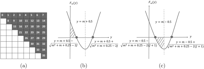
## Mathematical Diagrams: Grid and Function Plots ### Overview The image contains three distinct panels labeled (a), (b), and (c). Panel (a) is a numerical grid. Panels (b) and (c) are mathematical plots of a function \( F_m(y) \) against a variable \( y \), showing parabolic curves, specific points, and shaded regions defined by complex algebraic expressions. ### Components/Axes * **Panel (a):** A grid with 8 columns (labeled 0 through 7 at the top) and 6 rows. Cells contain integers. * **Panels (b) and (c):** * **Vertical Axis:** Labeled \( F_m(y) \). * **Horizontal Axis:** Labeled \( y \). * **Key Lines:** A vertical dashed line at \( y = m + 0.5 \) in (b) and at \( y = m - 0.5 \) in (c). * **Curves:** Both plots show an upward-opening parabola intersecting the horizontal axis at two points. * **Shaded Regions:** Hatched areas under the curve, bounded by specific vertical lines. * **Labels:** Mathematical expressions define the boundaries of the shaded regions and the intersection points. ### Detailed Analysis **Panel (a): Numerical Grid** The grid is structured as follows (Row, Column): * **Row 1 (Top):** 0, 1, 2, 3, 4, 5, 6, 7 * **Row 2:** (Empty), 8, 9, 10, 11, 12, 13, 14 * **Row 3:** (Empty), (Empty), 15, 16, 17, 18, 19, 20 * **Row 4:** (Empty), (Empty), (Empty), 21, 22, 23, 24, 25 * **Row 5:** (Empty), (Empty), (Empty), (Empty), 26, 27, 28, 29 * **Row 6 (Bottom):** (Empty), (Empty), (Empty), (Empty), (Empty), 30, 31, 32, 33, 34, 35 * **Note:** The grid forms a lower triangular pattern of numbers from 0 to 35. **Panel (b): Function Plot with Center at \( m+0.5 \)** * **Trend:** The curve \( F_m(y) \) is a parabola opening upwards. * **Key Points:** The parabola intersects the y-axis at two points. The left intersection is labeled with the expression: \( y = m + 0.5 - \sqrt{m^2 + m + 0.25 - 2j} \) The right intersection is labeled: \( y = m + 0.5 + \sqrt{m^2 + m + 0.25 - 2j} \) * **Shaded Region:** A hatched area is under the left side of the parabola. It is bounded on the left by a vertical line at: \( y = m + 0.5 - \sqrt{m^2 + m + 0.25 - 2j} \) and on the right by the vertical dashed line at \( y = m + 0.5 \). **Panel (c): Function Plot with Center at \( m-0.5 \)** * **Trend:** The curve \( F_m(y) \) is again an upward-opening parabola. * **Key Points:** The parabola intersects the y-axis at two points. The left intersection is labeled: \( y = m - 0.5 - \sqrt{m^2 + m + 0.25 - 2(j+1)} \) The right intersection is labeled: \( y = m - 0.5 + \sqrt{m^2 + m + 0.25 - 2(j+1)} \) * **Shaded Region:** A hatched area is under the right side of the parabola. It is bounded on the left by the vertical dashed line at \( y = m - 0.5 \) and on the right by a vertical line at: \( y = m - 0.5 + \sqrt{m^2 + m + 0.25 - 2(j+1)} \). ### Key Observations 1. **Symmetry:** The expressions for the intersection points in both (b) and (c) are symmetric around their respective central vertical lines (\( m+0.5 \) and \( m-0.5 \)). 2. **Parameter Shift:** The primary difference between plots (b) and (c) is the shift of the central axis from \( m+0.5 \) to \( m-0.5 \) and the increment of the parameter \( j \) to \( j+1 \) inside the square root term. 3. **Shaded Area Location:** The shaded region in (b) is to the *left* of the central axis, while in (c) it is to the *right*. 4. **Grid Pattern:** The grid in (a) shows a clear diagonal fill pattern, suggesting a structured indexing or mapping scheme. ### Interpretation These diagrams appear to illustrate concepts from probability theory or statistical mechanics, likely related to cumulative distribution functions (\( F_m(y) \)) for a discrete or continuous variable. * **Panels (b) and (c)** visually represent the calculation of probabilities (shaded areas) for a variable \( y \) under a quadratic (parabolic) function. The expressions under the square roots, \( m^2 + m + 0.25 - 2j \) and \( m^2 + m + 0.25 - 2(j+1) \), resemble discriminants or variance-related terms. The shift from \( j \) to \( j+1 \) and the change in the central axis suggest these plots compare two adjacent states or outcomes in a sequence. * **Panel (a)** likely serves as a reference table, possibly for values of \( j \) or another index, mapped onto a 2D grid. The triangular arrangement could indicate a constraint, such as \( j \) being a function of row and column indices. * **Overall Connection:** The figures together may explain how a probability mass or cumulative probability is distributed around a mean value (\( m \pm 0.5 \)) and how this distribution changes with a parameter \( j \). The grid provides the discrete parameter space, while the plots show the continuous functional form and associated probabilities.

## Grid and Function Graphs: Mathematical Representation ### Overview The image consists of three components: 1. A numerical grid (a) with shaded cells 2. Two function graphs (b and c) depicting Fₘ(y) with mathematical equations 3. Vertical dashed lines and shaded regions indicating specific mathematical relationships ### Components/Axes **Grid (a):** - **Rows:** Labeled 0–7 (vertical axis) - **Columns:** Labeled 8–35 (horizontal axis) - **Shaded Cells:** - Row 0: Columns 8–14 - Row 1: Columns 15–20 - Row 2: Columns 21–25 - Row 3: Columns 26–29 - Row 4: Columns 30–32 - Row 5: Columns 33–34 - Row 6: Column 35 **Graphs (b and c):** - **Y-axis:** Fₘ(y) (function value) - **X-axis:** y (variable) - **Vertical Dashed Line:** y = m (critical threshold) - **Legend:** Shaded region labeled "Fₘ(y)" ### Detailed Analysis **Grid (a):** - Shaded cells form a stepped pattern, increasing in column count per row until row 3, then decreasing. - Total shaded cells: 35 (matches column 35 in row 6). **Graph (b):** - **Equations:** - Upper boundary: y = m + 0.5 + √(m² + m + 0.25 − 2J) - Lower boundary: y = m + 0.5 − √(m² + m + 0.25 − 2J) - **Shaded Region:** Between the two curves, symmetric about y = m + 0.5. - **Vertical Dashed Line:** At y = m, intersecting the shaded region. **Graph (c):** - **Equations:** - Upper boundary: y = m − 0.5 + √(m² + m + 0.25 − 2(J + 1)) - Lower boundary: y = m − 0.5 − √(m² + m + 0.25 − 2(J + 1)) - **Shaded Region:** Between the two curves, symmetric about y = m − 0.5. - **Vertical Dashed Line:** At y = m, intersecting the shaded region. ### Key Observations 1. **Grid Pattern:** Shaded cells suggest a hierarchical or tiered structure, with diminishing density in higher rows. 2. **Graph Symmetry:** Both graphs exhibit parabolic symmetry around their respective midlines (y = m ± 0.5). 3. **Parameter Sensitivity:** - Graph (b) uses J, while graph (c) uses J + 1, shifting the curves downward. - The square root terms imply constraints on J (e.g., m² + m + 0.25 − 2J ≥ 0). ### Interpretation - **Grid (a):** Likely represents a matrix or heatmap where shaded cells encode specific values (e.g., active states, thresholds). The stepped pattern may reflect a decay or prioritization mechanism. - **Graphs (b and c):** Model a function Fₘ(y) with parameter-dependent bounds. The shaded regions could represent allowable ranges or confidence intervals. - Graph (b) corresponds to J, while graph (c) adjusts for J + 1, suggesting iterative or incremental analysis. - The vertical dashed line (y = m) acts as a reference point, possibly a mean or critical value. - **Mathematical Relationships:** The equations highlight dependencies on m and J, with the square root terms introducing nonlinear constraints. This structure suggests a system where grid-based data (a) informs parameter choices (m, J) in the function graphs (b, c), with shaded regions visualizing solution spaces or valid ranges.