## Diagram: Comparison of CIM Models
### Overview
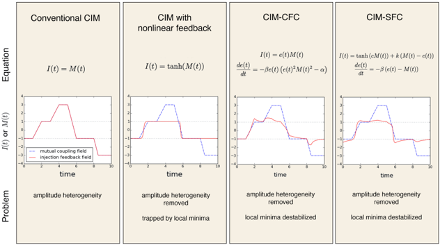
The image presents a comparative analysis of four different Coupled-Inhibitory Mutator (CIM) models: Conventional CIM, CIM with nonlinear feedback, CIM-CFC, and CIM-SFC. For each model, the image provides the governing equation, a plot illustrating the behavior of the mutual coupling field and injection feedback field over time, and a brief description of the problem addressed by the model.
### Components/Axes
* **Columns:** The image is divided into four columns, each representing a different CIM model.
* Column 1: Conventional CIM
* Column 2: CIM with nonlinear feedback
* Column 3: CIM-CFC
* Column 4: CIM-SFC
* **Rows:** The image is divided into three rows for each model:
* Row 1: Equation defining the model
* Row 2: Plot of I(t) or M(t) vs. time
* Row 3: Problem addressed by the model
* **Plots:** Each plot has the following axes:
* Y-axis: Labeled "I(t) or M(t)", ranging from -4 to 4 with tick marks at -3, -2, -1, 0, 1, 2, 3, and 4.
* X-axis: Labeled "time", ranging from 0 to 10 with tick marks at 2, 4, 6, 8, and 10.
* **Legend:** Located within each plot, indicating:
* Blue dashed line: "mutual coupling field"
* Red solid line: "injection feedback field"
### Detailed Analysis
**1. Conventional CIM**
* **Equation:** I(t) = M(t)
* **Plot:**
* The blue dashed line (mutual coupling field) starts at approximately -1, increases linearly to 1 at time = 2, then increases linearly to 3 at time = 4. It remains constant at 3 until time = 6, then decreases linearly to -1 at time = 8, and remains constant at -1 until time = 10.
* The red solid line (injection feedback field) is identical to the blue dashed line.
* **Problem:** amplitude heterogeneity
**2. CIM with nonlinear feedback**
* **Equation:** I(t) = tanh(M(t))
* **Plot:**
* The blue dashed line (mutual coupling field) is identical to the mutual coupling field in the Conventional CIM plot.
* The red solid line (injection feedback field) starts at approximately -0.8, increases to approximately 0.8 at time = 2, then increases to approximately 1 at time = 4. It remains constant at 1 until time = 6, then decreases to approximately -0.8 at time = 8, and remains constant at -0.8 until time = 10.
* **Problem:** amplitude heterogeneity removed, trapped by local minima
**3. CIM-CFC**
* **Equation:**
* I(t) = e(t)M(t)
* de(t)/dt = -βe(t)(e(t)^2M(t)^2 - α)
* **Plot:**
* The blue dashed line (mutual coupling field) is identical to the mutual coupling field in the Conventional CIM plot.
* The red solid line (injection feedback field) starts at approximately -0.8, increases to approximately 1.5 at time = 2, then increases to approximately 2 at time = 4. It decreases to approximately -1 at time = 6, and remains constant at -1 until time = 10.
* **Problem:** amplitude heterogeneity removed, local minima destabilized
**4. CIM-SFC**
* **Equation:**
* I(t) = tanh(cM(t)) + k(M(t) - e(t))
* de(t)/dt = -β(e(t) - M(t))
* **Plot:**
* The blue dashed line (mutual coupling field) is identical to the mutual coupling field in the Conventional CIM plot.
* The red solid line (injection feedback field) starts at approximately -0.8, increases to approximately 1.5 at time = 2, then increases to approximately 1.5 at time = 4. It decreases to approximately -1 at time = 6, and remains constant at -1 until time = 10.
* **Problem:** amplitude heterogeneity removed, local minima destabilized
### Key Observations
* The "mutual coupling field" (blue dashed line) is identical across all four models.
* The "injection feedback field" (red solid line) varies significantly between the models, reflecting the different equations and feedback mechanisms.
* The Conventional CIM model has identical mutual coupling and injection feedback fields.
* The CIM with nonlinear feedback model compresses the amplitude of the injection feedback field due to the tanh function.
* The CIM-CFC and CIM-SFC models show a more complex behavior of the injection feedback field, with a sharper decrease after time = 6.
### Interpretation
The image illustrates how different mathematical formulations of the CIM model affect the behavior of the injection feedback field. The Conventional CIM model serves as a baseline, where the injection feedback field mirrors the mutual coupling field. The subsequent models introduce modifications to address specific problems, such as amplitude heterogeneity and the trapping of local minima. The nonlinear feedback model compresses the amplitude, while the CIM-CFC and CIM-SFC models destabilize local minima, potentially leading to more dynamic and adaptable system behavior. The equations provided offer a mathematical description of these behaviors, while the plots provide a visual representation of the system's response over time.