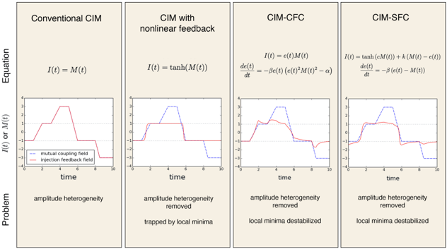
## Technical Diagram: Comparison of CIM Variants ### Overview The image is a technical comparison chart divided into four vertical panels, each detailing a different variant of a system referred to as "CIM". The panels are arranged from left to right, showing a progression from a conventional method to more advanced variants with nonlinear feedback mechanisms. Each panel contains three consistent sections: a mathematical equation, a corresponding time-series graph, and a statement of the associated problem. ### Components/Axes **Panel Structure (Left to Right):** 1. **Panel 1 Header:** "Conventional CIM" 2. **Panel 2 Header:** "CIM with nonlinear feedback" 3. **Panel 3 Header:** "CIM-CFC" 4. **Panel 4 Header:** "CIM-SFC" **Common Graph Elements (Present in all four panels):** * **Y-axis Label:** `I(t) or M(t)` (Positioned vertically on the left side of each graph). * **X-axis Label:** `time` (Positioned below each graph). * **X-axis Scale:** Linear, marked from 0 to 10 with major ticks at 0, 2, 4, 6, 8, 10. * **Y-axis Scale:** Linear, marked from -4 to 4 with major ticks at -4, -2, 0, 2, 4. * **Legend (Bottom-left of each graph):** * A solid red line is labeled: `mutual coupling field` * A dashed blue line is labeled: `injection feedback field` **Equations (Top section of each panel):** 1. **Conventional CIM:** `I(t) = M(t)` 2. **CIM with nonlinear feedback:** `I(t) = tanh(M(t))` 3. **CIM-CFC:** Two equations are presented: * `I(t) = ε(t)M(t)` * `dε(t)/dt = -βε(t){ε(t)²M(t)² - α}` 4. **CIM-SFC:** Two equations are presented: * `I(t) = tanh(ε(t)M(t)) + k(M(t) - ε(t))` * `dε(t)/dt = -β(ε(t) - M(t))` **Problem Statements (Bottom section of each panel):** 1. **Conventional CIM:** `amplitude heterogeneity` 2. **CIM with nonlinear feedback:** `amplitude heterogeneity removed` / `trapped by local minima` 3. **CIM-CFC:** `amplitude heterogeneity removed` / `local minima destabilized` 4. **CIM-SFC:** `amplitude heterogeneity removed` / `local minima destabilized` ### Detailed Analysis **Graph 1: Conventional CIM** * **Trend:** The red line (`mutual coupling field`) follows a trapezoidal pulse shape. It rises linearly from 0 to 2 between t=0 and t=2, holds steady at 2 until t=4, rises again to 4 between t=4 and t=5, holds at 4 until t=6, then falls linearly back to 0 by t=8, and remains at 0. * **Data Points (Approximate):** (0,0), (2,2), (4,2), (5,4), (6,4), (8,0), (10,0). * **Note:** The blue dashed line (`injection feedback field`) is not visible, implying it is either zero or identical to the red line. **Graph 2: CIM with nonlinear feedback** * **Trend:** The red line (`mutual coupling field`) is a smoothed, lower-amplitude version of the trapezoid. It rises to about 1.5 by t=2, holds, rises to about 2.5 by t=5, holds, then falls to 0 by t=8. The blue dashed line (`injection feedback field`) is now visible and follows a similar but distinct path, rising to about 3 by t=4, holding, then falling to -2 by t=9. * **Key Relationship:** The red line appears to be a `tanh`-compressed version of the blue line, consistent with the equation `I(t) = tanh(M(t))`. **Graph 3: CIM-CFC** * **Trend:** The blue dashed line (`injection feedback field`) follows a similar path to Panel 2. The red line (`mutual coupling field`) now exhibits more complex, oscillatory behavior, especially during the rising and falling edges. It shows small peaks and valleys around the main trend, suggesting the influence of the dynamic `ε(t)` term. * **Key Relationship:** The red line is now a product of `ε(t)` and the blue line (`I(t) = ε(t)M(t)`), where `ε(t)` itself is changing over time according to its differential equation. **Graph 4: CIM-SFC** * **Trend:** The blue dashed line (`injection feedback field`) is again similar. The red line (`mutual coupling field`) shows a smoother response than in CIM-CFC but with a noticeable offset or lag compared to the blue line, particularly during the plateau phases. It also dips slightly below zero after t=8. * **Key Relationship:** The red line is a more complex function of both `ε(t)M(t)` and the difference `(M(t) - ε(t))`, with `ε(t)` driven to track `M(t)`. ### Key Observations 1. **Progression of Complexity:** The system evolves from a simple linear relationship (Panel 1) to a static nonlinearity (Panel 2), and finally to two variants (Panels 3 & 4) with dynamic, adaptive elements (`ε(t)`). 2. **Problem-Solution Trade-off:** Each step solves the previous problem but introduces a new one. Nonlinear feedback removes amplitude heterogeneity but traps the system in local minima. The CFC and SFC variants destabilize those local minima to escape them. 3. **Visual Signature of Dynamics:** The presence of oscillations (CIM-CFC) or tracking lag (CIM-SFC) in the red line are direct visual manifestations of the underlying differential equations governing `ε(t)`. 4. **Legend Consistency:** The color coding (red for `mutual coupling field`/`I(t)`, blue for `injection feedback field`/`M(t)`) is consistent across all panels, allowing for direct comparison of how the relationship between these two signals changes. ### Interpretation This diagram illustrates a common engineering design trajectory: starting with a simple, intuitive model, identifying its failure modes (amplitude heterogeneity), and iteratively adding complexity to address those failures. * **Conventional CIM** represents a baseline, direct-coupling system. Its flaw is that the output (`I(t)`) directly mirrors the input's (`M(t)`) amplitude variations. * **CIM with nonlinear feedback** uses a `tanh` function to squash the output, standardizing amplitudes. However, this creates a smooth but "bumpy" optimization landscape with many local minima where the system can get stuck. * **CIM-CFC (Coupling Feedback Control)** and **CIM-SFC (State Feedback Control)** introduce a dynamic gain factor `ε(t)`. This gain adapts over time based on the system's state, effectively "shaking" or "smoothing" the optimization landscape to prevent trapping. The different equations for `dε(t)/dt` represent two distinct control strategies for achieving this destabilization of local minima. The graphs provide a visual proof of concept: the advanced methods (CFC, SFC) successfully modify the system's temporal response (`I(t)`) in a more complex way than simple clipping, which is the intended mechanism for improving performance in whatever larger computational or control task this CIM system is part of. The trade-off is increased mathematical and potentially computational complexity.