## Chart/Diagram Type: Comparative Analysis of Control Mechanisms in CIM Systems
### Overview
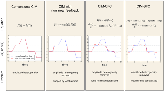
The image presents four panels comparing different control mechanisms for Current-Induced Magnetization (CIM) systems. Each panel includes an equation, a time-series graph, and a problem statement. The graphs visualize the behavior of mutual coupling fields (blue) and injection feedback fields (red) over time, with annotations highlighting key issues like amplitude heterogeneity and local minima.
---
### Components/Axes
1. **Panels**:
- **Panel 1**: Conventional CIM
- Equation: $ I(t) = M(t) $
- Problem: Amplitude heterogeneity
- **Panel 2**: CIM with nonlinear feedback
- Equation: $ I(t) = \tanh(M(t)) $
- Problem: Amplitude heterogeneity removed, trapped by local minima
- **Panel 3**: CIM-CFC
- Equation: $ I(t) = e(t)M(t) $, $ \frac{de(t)}{dt} = -\beta e(t)\left( (e(t))^2M(t)^2 - \alpha \right) $
- Problem: Amplitude heterogeneity removed, local minima destabilized
- **Panel 4**: CIM-SFC
- Equation: $ I(t) = \tanh(cM(t)) + k(M(t)) - e(t) $, $ \frac{de(t)}{dt} = -\beta(e(t) - M(t)) $
- Problem: Amplitude heterogeneity removed, local minima destabilized
2. **Graphs**:
- **X-axis**: Time (0–10 units)
- **Y-axis**: $ I(t) $ or $ M(t) $ (amplitude values, approximately -4 to 4)
- **Legends**:
- Blue line: Mutual coupling field
- Red line: Injection feedback field
- **Placement**: Legends are positioned at the bottom-left of each graph.
3. **Annotations**:
- Problem statements are placed at the bottom of each panel.
---
### Detailed Analysis
#### Panel 1: Conventional CIM
- **Graph**:
- Mutual coupling field (blue) peaks at ~2.5, drops sharply after ~3.5.
- Injection feedback field (red) peaks at ~3.5, drops sharply after ~4.
- Both lines exhibit significant amplitude heterogeneity (large fluctuations).
- **Problem**: Amplitude heterogeneity is evident in both fields.
#### Panel 2: CIM with Nonlinear Feedback
- **Graph**:
- Mutual coupling field (blue) stabilizes after a peak (~2.5), with reduced fluctuations.
- Injection feedback field (red) drops to zero after ~3.5.
- Amplitude heterogeneity is reduced but trapped by local minima (flat regions).
- **Problem**: Local minima trap the system, limiting dynamic response.
#### Panel 3: CIM-CFC
- **Graph**:
- Mutual coupling field (blue) fluctuates but with smaller peaks (~1.5–2).
- Injection feedback field (red) shows irregular oscillations, destabilizing local minima.
- **Problem**: Local minima are destabilized, but amplitude heterogeneity is mitigated.
#### Panel 4: CIM-SFC
- **Graph**:
- Mutual coupling field (blue) peaks at ~2.5, with minor fluctuations.
- Injection feedback field (red) stabilizes after ~3.5, with reduced oscillations.
- Both fields exhibit smoother behavior compared to earlier panels.
- **Problem**: Local minima are destabilized, but amplitude heterogeneity is resolved.
---
### Key Observations
1. **Amplitude Heterogeneity**:
- Present in Panel 1 (large fluctuations).
- Reduced in Panels 2–4 but introduces trade-offs (local minima in Panel 2, destabilization in Panels 3–4).
2. **Local Minima**:
- Trapped in Panel 2 (flat regions in red line).
- Destabilized in Panels 3–4 (irregular oscillations in red line).
3. **Equation Complexity**:
- Nonlinear feedback (Panel 2) simplifies the system but introduces stability issues.
- CIM-CFC and CIM-SFC use differential equations to actively manage feedback, improving stability at the cost of complexity.
---
### Interpretation
The progression from conventional CIM to CIM-SFC demonstrates iterative improvements in controlling amplitude heterogeneity. However, each modification introduces new challenges:
- **Nonlinear feedback** (Panel 2) reduces heterogeneity but traps the system in local minima, limiting adaptability.
- **CIM-CFC** (Panel 3) destabilizes local minima but requires precise tuning of parameters ($ \beta, \alpha $) to avoid instability.
- **CIM-SFC** (Panel 4) balances stability and heterogeneity removal but relies on additional terms ($ k(M(t)) $) to manage feedback.
The graphs suggest that advanced control mechanisms (CIM-CFC, CIM-SFC) prioritize dynamic stability over simplicity, reflecting a trade-off between mathematical complexity and system performance. The destabilization of local minima in later panels may enhance responsiveness but risks overshooting or oscillations, requiring further optimization.