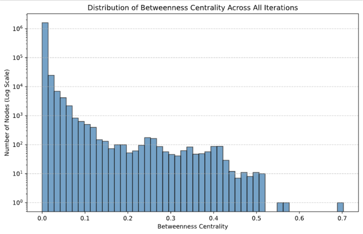
## Histogram: Distribution of Betweenness Centrality Across All Iterations ### Overview This image is a histogram visualizing the frequency distribution of "Betweenness Centrality" values for a set of nodes across multiple iterations. The chart utilizes a logarithmic scale on the Y-axis to accommodate the extreme disparity in node counts, ranging from a few nodes at high centrality values to over a million nodes at very low centrality values. ### Components/Axes * **Title:** "Distribution of Betweenness Centrality Across All Iterations" (Centered at the top). * **Y-Axis:** Labeled "Number of Nodes (Log Scale)". The scale is logarithmic, with major grid lines at powers of 10 ($10^0$, $10^1$, $10^2$, $10^3$, $10^4$, $10^5$, $10^6$). * **X-Axis:** Labeled "Betweenness Centrality". The scale is linear, ranging from 0.0 to 0.7, with major tick marks every 0.1 units. * **Data Representation:** Blue vertical bars representing the count of nodes falling into specific centrality bins. The bin width appears to be approximately 0.01 to 0.02 units. ### Detailed Analysis The distribution exhibits a heavy right-skew (or "long tail"), which is typical for network centrality metrics. * **The Primary Peak (0.0 - 0.02):** The first bin, representing nodes with near-zero betweenness centrality, is the tallest, extending above the $10^6$ line (approximately 1.5 million nodes). * **The Rapid Decline (0.02 - 0.15):** There is a steep, exponential-like decay in the number of nodes as centrality increases from 0.02 to 0.15. * At ~0.02-0.04, the count drops to approximately $2 \times 10^4$. * At ~0.06-0.08, the count drops further to approximately $4 \times 10^3$. * By ~0.15, the count has fallen to roughly $10^2$ (100 nodes). * **Mid-Range Fluctuations (0.2 - 0.45):** The decline levels off into a "long tail" with several minor fluctuations: * **Local Plateau/Bump (0.24 - 0.27):** There is a noticeable local increase in frequency, with bars reaching slightly above $10^2$. * **Local Plateau/Bump (0.38 - 0.42):** Another distinct cluster of nodes appears here, with frequencies also reaching near $10^2$. * **The Sparse Tail (0.45 - 0.7):** * The frequency drops significantly after 0.42, falling to near $10^1$ (10 nodes) and below. * **Gaps:** There are distinct gaps in the data where no nodes exist, specifically between ~0.52 and 0.55, and between ~0.58 and 0.70. * **Outliers:** There are isolated single nodes (or very small counts) at approximately 0.56, 0.57, and 0.70. ### Key Observations * **Extreme Skew:** The vast majority of nodes in the dataset have extremely low betweenness centrality, indicating they are peripheral nodes that do not lie on many shortest paths. * **Logarithmic Necessity:** The use of a log scale is essential here; without it, the bars representing the high-centrality nodes (the tail) would be invisible, appearing as flat lines against the massive count of the first bin. * **Structural Implications:** The presence of secondary "bumps" at 0.25 and 0.4 suggests the network may have specific structural sub-components or "bridge" nodes that appear with higher-than-random frequency, rather than a perfectly smooth decay. ### Interpretation This data is characteristic of a **scale-free network** or a network with a strong "hub-and-spoke" architecture. 1. **Peripheral Dominance:** The overwhelming concentration of nodes at the 0.0-0.02 range suggests that most nodes in this system are "leaves" or peripheral members with very little influence over information flow or connectivity between other nodes. 2. **Bridge Nodes:** The nodes with higher centrality (the tail) are the critical "bridges" or "hubs." Even though they are few in number, they are essential for the connectivity of the entire network. 3. **Structural Anomalies:** The gaps in the tail (e.g., the absence of nodes between 0.52 and 0.55) suggest that there are "forbidden" or unreachable centrality values in this specific network topology. This could indicate that the network is constrained by specific rules of growth or iteration, preventing nodes from achieving certain intermediate levels of centrality. 4. **Peircean Investigative Note:** The secondary modes at 0.25 and 0.4 are the most interesting features. They deviate from a standard power-law decay. This implies that the "iterations" mentioned in the title likely involve a process (perhaps a specific algorithm or growth rule) that actively promotes the creation of nodes with these specific centrality values, rather than them occurring purely by chance.