## Histogram: Distribution of Betweenness Centrality
### Overview
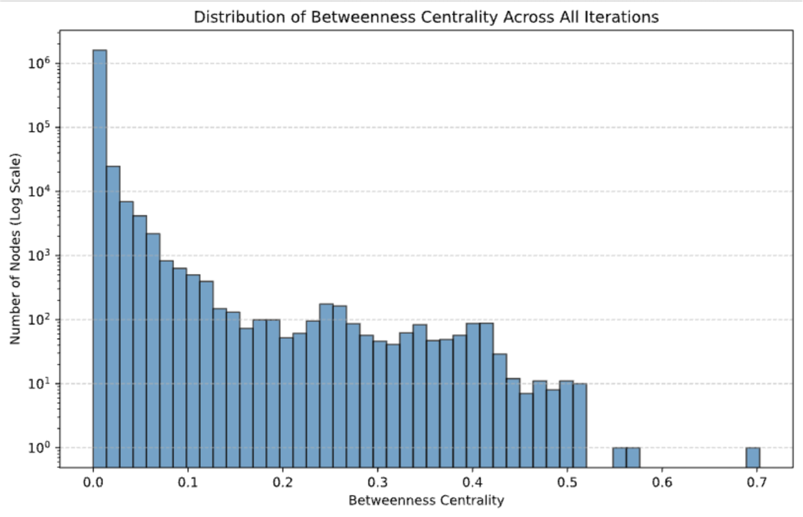
This image is a histogram displaying the frequency distribution of a network metric called "Betweenness Centrality." The chart utilizes a linear scale for the x-axis and a logarithmic scale (base 10) for the y-axis. The data is represented by contiguous vertical blue bars with black outlines. The language present in the image is entirely English.
### Components/Axes
**1. Header Region (Top Center)**
* **Chart Title:** "Distribution of Betweenness Centrality Across All Iterations"
**2. Y-Axis (Left Edge)**
* **Label:** "Number of Nodes (Log Scale)" (Oriented vertically, reading bottom-to-top).
* **Scale:** Logarithmic (Base 10).
* **Tick Markers:** $10^0, 10^1, 10^2, 10^3, 10^4, 10^5, 10^6$.
* **Gridlines:** Light gray, dashed horizontal lines extend from each major tick mark across the main chart area.
**3. X-Axis (Bottom Edge)**
* **Label:** "Betweenness Centrality"
* **Scale:** Linear.
* **Tick Markers:** 0.0, 0.1, 0.2, 0.3, 0.4, 0.5, 0.6, 0.7.
**4. Main Chart Area (Center)**
* **Data Series:** A single series of light blue bars representing the frequency of nodes falling into specific betweenness centrality bins. The bin width appears to be approximately ~0.014 units wide (roughly 7 bars per 0.1 interval).
### Detailed Analysis
**Visual Trend Verification:**
The overall visual trend is a massive right-skewed (heavy-tailed) distribution. The line formed by the tops of the bars slopes sharply downward from the extreme left, indicating that the vast majority of nodes have a betweenness centrality at or very near 0.0. As the x-value increases, the y-value drops precipitously by several orders of magnitude. However, the descent is not perfectly smooth; there are distinct secondary "bumps" or local maxima in the mid-ranges, followed by a sparse scattering of isolated outliers at the extreme right end of the x-axis.
**Data Extraction (Approximate Values):**
Due to the logarithmic scale and visual estimation, values are approximate ($\sim$).
* **The Primary Peak (0.0 to 0.05):**
* The first bin (starting at 0.0) contains the absolute maximum, exceeding the $10^6$ line. Estimated value: $\sim 1.5 \times 10^6$ nodes.
* The second bin drops sharply to $\sim 2.5 \times 10^4$.
* The frequency continues to decay rapidly through 0.1, dropping to $\sim 5 \times 10^2$.
* **The Mid-Range Plateau and Bumps (0.15 to 0.45):**
* Between 0.15 and 0.25, the frequency fluctuates between $\sim 5 \times 10^1$ and $10^2$.
* **Local Maximum 1:** A distinct spike occurs around x = 0.26, reaching $\sim 1.8 \times 10^2$.
* The frequency dips again around x = 0.32 to $\sim 4 \times 10^1$.
* **Local Maximum 2:** Another distinct spike occurs around x = 0.41, reaching $\sim 9 \times 10^1$.
* **The Tail and Outliers (0.45 to 0.7):**
* After x = 0.45, the contiguous bars drop to the $10^1$ range and below.
* The contiguous distribution ends around x = 0.52.
* **Outlier 1:** A single bar at x $\sim 0.55$, resting exactly on the $10^0$ line (1 node).
* **Outlier 2:** A single bar at x $\sim 0.57$, resting exactly on the $10^0$ line (1 node).
* **Outlier 3:** A single bar at x $\sim 0.69$, resting exactly on the $10^0$ line (1 node).
**Reconstructed Representative Data Table:**
*(Note: Bins are approximated based on visual width; Y-values are estimated from the log scale).*
| Centrality Range (Approx X) | Number of Nodes (Approx Y) | Visual Characteristic |
| :--- | :--- | :--- |
| 0.000 - 0.014 | $1,500,000$ | Absolute Maximum |
| 0.014 - 0.028 | $25,000$ | Sharp decay |
| 0.085 - 0.100 | $600$ | Continued decay |
| 0.185 - 0.210 | $100$ | Plateau |
| 0.250 - 0.270 | $180$ | Local Maximum |
| 0.310 - 0.330 | $40$ | Local Minimum |
| 0.400 - 0.420 | $90$ | Local Maximum |
| 0.500 - 0.520 | $10$ | End of contiguous tail |
| $\sim 0.55$ | $1$ ($10^0$) | Isolated Outlier |
| $\sim 0.57$ | $1$ ($10^0$) | Isolated Outlier |
| $\sim 0.69$ | $1$ ($10^0$) | Extreme Outlier |
### Key Observations
1. **Extreme Concentration at Zero:** Over 1 million nodes have a betweenness centrality near zero, while all other bins combined contain only a fraction of that amount.
2. **Logarithmic Decay:** The use of a log scale on the y-axis is necessary to even see the data beyond x=0.05. The drop from the first bin to the outliers represents a difference of six orders of magnitude.
3. **Structural Bumps:** The presence of secondary peaks around 0.26 and 0.41 indicates that while high centrality is rare, there are specific structural roles or network tiers that group nodes into these specific centrality bands.
4. **The "Super-Hub":** There is exactly one node with a centrality near 0.7, making it the most critical bridge in the entire network by a significant margin compared to the next highest nodes (~0.57).
### Interpretation
**What the data means:**
Betweenness centrality measures how often a node acts as a bridge along the shortest path between two other nodes. A value of 0 means the node is never on a shortest path (typically "leaf" nodes at the edges of a network). A high value indicates a "bottleneck" or "hub" that controls the flow of information across the network.
**Reading between the lines (Peircean investigative analysis):**
* **Network Topology:** This histogram strongly suggests a highly centralized, scale-free, or "hub-and-spoke" network topology. The fact that over $10^6$ nodes have near-zero centrality implies a massive periphery of disconnected or single-connection users/entities.
* **Vulnerability:** The network is highly reliant on a very small number of nodes. The single node at ~0.7 and the few nodes between 0.4 and 0.6 are critical points of failure. If these nodes are removed, the network would likely shatter into disconnected components, as they are the primary bridges connecting the millions of peripheral nodes.
* **The "Iterations" Context:** The title mentions "Across All Iterations." This suggests this data might be aggregated from a simulation, a dynamic network changing over time, or an algorithm (like a random walk or routing protocol) running multiple times. The secondary "bumps" (at 0.26 and 0.41) might represent specific phases of the iteration or distinct hierarchical layers within the network's core that consistently emerge across these iterations.