\n
## Histogram: Distribution of Betweenness Centrality Across All Iterations
### Overview
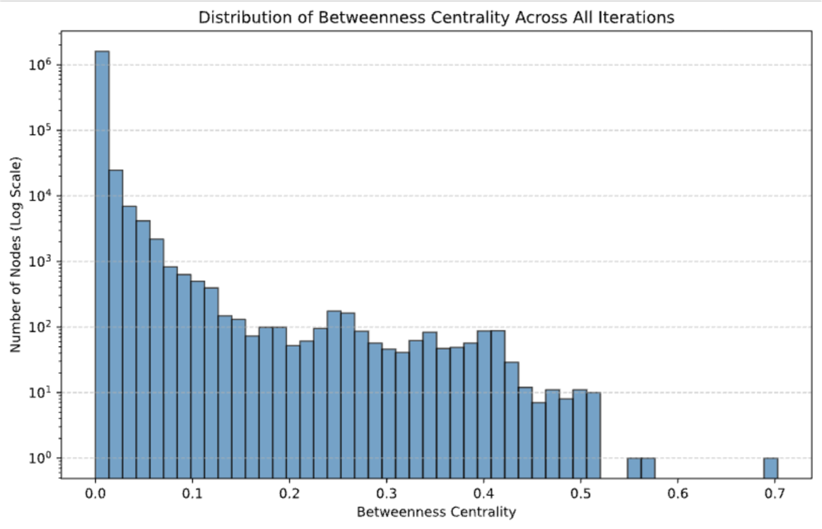
The image presents a histogram visualizing the distribution of betweenness centrality values across all iterations. The y-axis is displayed on a logarithmic scale. The distribution is heavily skewed to the left, indicating that most nodes have low betweenness centrality.
### Components/Axes
* **Title:** "Distribution of Betweenness Centrality Across All Iterations" (centered at the top)
* **X-axis Label:** "Betweenness Centrality" (centered at the bottom)
* Scale: Ranges from approximately 0.0 to 0.7, with markings at 0.0, 0.1, 0.2, 0.3, 0.4, 0.5, 0.6, and 0.7.
* **Y-axis Label:** "Number of Nodes (Log Scale)" (left side)
* Scale: Logarithmic, with markings at 10⁰, 10¹, 10², 10³, 10⁴, 10⁵, and 10⁶.
* **Histogram Bars:** Represent the frequency of nodes within specific betweenness centrality ranges. The bars are colored in a light blue/grey.
### Detailed Analysis
The histogram shows a rapid decrease in the number of nodes as betweenness centrality increases.
* **Betweenness Centrality 0.0 - 0.05:** Approximately 1.5 x 10⁶ nodes.
* **Betweenness Centrality 0.05 - 0.1:** Approximately 6 x 10⁵ nodes.
* **Betweenness Centrality 0.1 - 0.15:** Approximately 2.5 x 10⁵ nodes.
* **Betweenness Centrality 0.15 - 0.2:** Approximately 1 x 10⁵ nodes.
* **Betweenness Centrality 0.2 - 0.25:** Approximately 5 x 10⁴ nodes.
* **Betweenness Centrality 0.25 - 0.3:** Approximately 3 x 10⁴ nodes.
* **Betweenness Centrality 0.3 - 0.35:** Approximately 2 x 10⁴ nodes.
* **Betweenness Centrality 0.35 - 0.4:** Approximately 1.5 x 10⁴ nodes.
* **Betweenness Centrality 0.4 - 0.45:** Approximately 1 x 10⁴ nodes.
* **Betweenness Centrality 0.45 - 0.5:** Approximately 7 x 10³ nodes.
* **Betweenness Centrality 0.5 - 0.55:** Approximately 2 x 10³ nodes.
* **Betweenness Centrality 0.55 - 0.6:** Approximately 5 x 10² nodes.
* **Betweenness Centrality 0.6 - 0.65:** Approximately 1 x 10² nodes.
* **Betweenness Centrality 0.65 - 0.7:** Approximately 2 x 10¹ nodes.
The trend is a steep decline in node count with increasing betweenness centrality. The distribution appears to be approximately exponential.
### Key Observations
* The vast majority of nodes have very low betweenness centrality (less than 0.2).
* There are very few nodes with high betweenness centrality (greater than 0.5).
* The logarithmic scale on the y-axis is crucial for visualizing the distribution, as the differences in node counts are significant.
### Interpretation
This data suggests that the network is characterized by a few highly central nodes and many peripheral nodes. The high concentration of nodes with low betweenness centrality indicates that most nodes do not lie on many shortest paths between other nodes in the network. This could imply a hierarchical structure or a network with a core-periphery organization. The few nodes with high betweenness centrality likely act as critical connectors within the network, and their removal could significantly disrupt network connectivity. The shape of the distribution is consistent with scale-free networks, where a small number of nodes have a disproportionately large number of connections. The use of all iterations suggests that this distribution is stable over time, or represents an average state of the network.