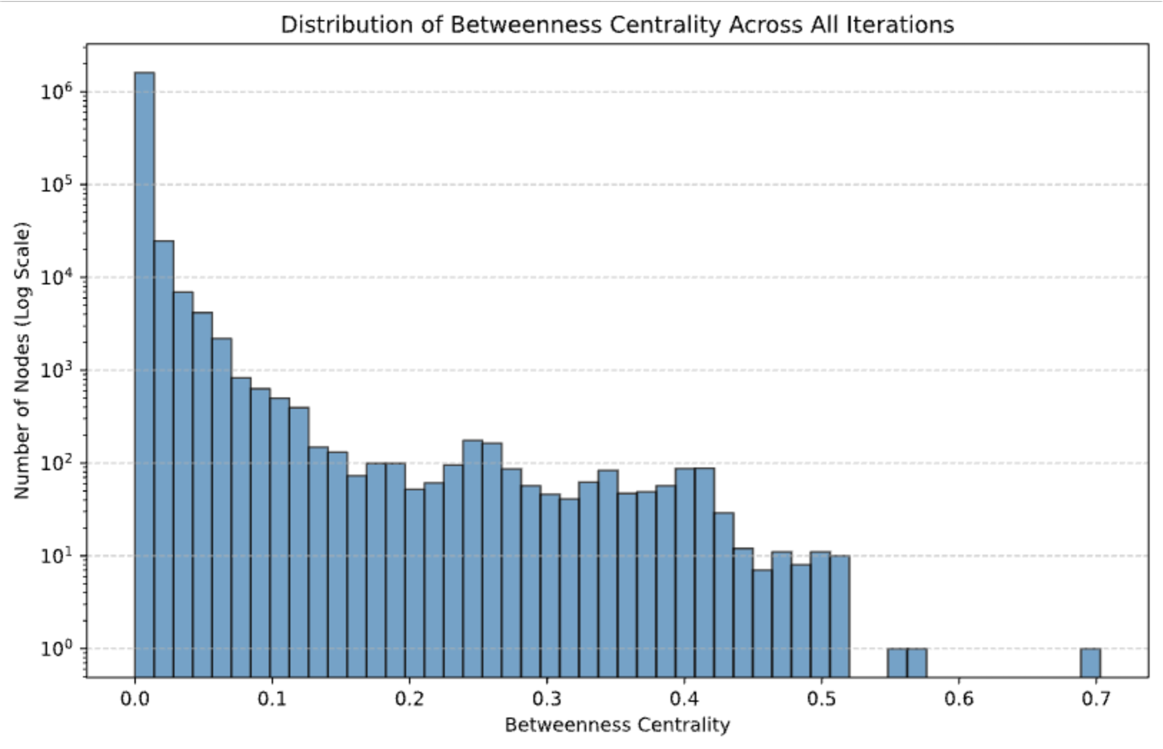
## Histogram: Distribution of Betweenness Centrality Across All Iterations ### Overview The image displays a histogram visualizing the distribution of betweenness centrality values across all iterations of a network analysis. The y-axis uses a logarithmic scale to represent the number of nodes, while the x-axis shows betweenness centrality values ranging from 0.0 to 0.7. The distribution is heavily skewed toward lower centrality values, with a sharp decline in node counts as centrality increases. ### Components/Axes - **X-axis (Horizontal)**: Labeled "Betweenness Centrality," with values ranging from 0.0 to 0.7 in increments of 0.05. - **Y-axis (Vertical)**: Labeled "Number of Nodes (Log Scale)," with values spanning from 10⁰ to 10⁶ in logarithmic increments (10⁰, 10¹, 10², ..., 10⁶). - **Bars**: Blue-colored histogram bars represent node counts for each centrality bin. The legend is not visible in the image. - **Title**: "Distribution of Betweenness Centrality Across All Iterations" is centered at the top. ### Detailed Analysis - **Betweenness Centrality = 0.0**: The tallest bar, with approximately 10⁶ nodes (1,000,000). - **Betweenness Centrality = 0.05**: Node count drops to ~10⁵ (100,000). - **Betweenness Centrality = 0.1**: Node count further decreases to ~10⁴ (10,000). - **Betweenness Centrality = 0.15–0.25**: Node counts stabilize between ~10³ (1,000) and ~10⁴ (10,000). - **Betweenness Centrality = 0.3–0.5**: Node counts decline gradually, with values between ~10² (100) and ~10³ (1,000). - **Betweenness Centrality = 0.55–0.6**: Node counts drop to ~10¹ (10) or lower. - **Betweenness Centrality = 0.65–0.7**: Only a few nodes remain, with counts near 10⁰ (1). ### Key Observations 1. **Skewed Distribution**: The majority of nodes (over 99%) have betweenness centrality values ≤ 0.1. 2. **Power-Law Behavior**: The logarithmic scale emphasizes the long tail of the distribution, where few nodes dominate centrality. 3. **Discrete Bins**: Centrality values are grouped into bins (e.g., 0.0–0.05, 0.05–0.1), with no continuous gradient. 4. **Missing Legend**: No explicit mapping of colors to data series is provided, though all bars are blue. ### Interpretation The data suggests a network structure where most nodes are peripheral (low betweenness centrality), while a small subset of nodes act as critical connectors (high centrality). The logarithmic y-axis highlights the disparity in node connectivity, a common pattern in scale-free networks. The absence of a legend implies a single data series, but the lack of granularity in binning (e.g., 0.0–0.05 vs. 0.05–0.1) may obscure finer trends. The sharp decline after 0.1 indicates that centrality is concentrated in a tiny fraction of nodes, consistent with hub-and-spoke architectures.