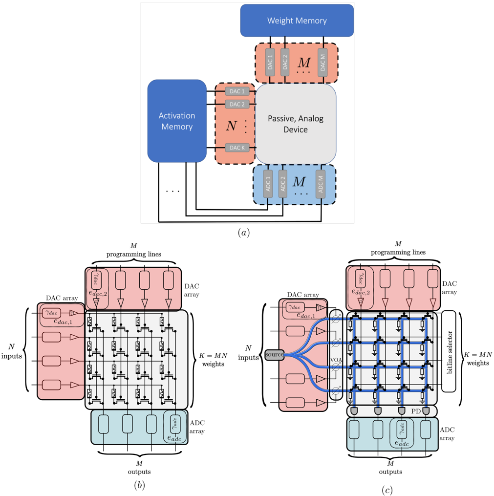
## Diagram: Analog Computing Core Architectures ### Overview The image presents three interconnected technical diagrams illustrating the architecture of an analog computing core, likely for neural network acceleration. The diagrams progress from a high-level system view (a) to two detailed circuit-level implementations (b and c). The system uses digital-to-analog converters (DACs) and analog-to-digital converters (ADCs) to interface digital memory with a passive, analog computational device. ### Components/Axes The image is divided into three distinct panels, labeled (a), (b), and (c). **Panel (a) - System Block Diagram:** * **Primary Blocks:** * **Weight Memory** (Blue, top): Stores the model weights. * **Activation Memory** (Blue, left): Stores the input activation data. * **Passive, Analog Device** (Grey, center): The core computational element where analog multiplication and summation occur. * **Interface Blocks:** * **DAC Array (N)** (Orange, left of center): A set of `N` Digital-to-Analog Converters (labeled DAC 1, DAC 2, ... DAC K) converting digital activations to analog signals. * **DAC Array (M)** (Orange, top of center): A set of `M` DACs (labeled DAC 1, DAC 2, ... DAC M) converting digital weights to analog programming signals. * **ADC Array (M)** (Light Blue, bottom of center): A set of `M` Analog-to-Digital Converters (labeled ADC 1, ADC 2, ... ADC M) converting analog output currents back to digital. * **Data Flow:** Digital data flows from memories through DACs to the analog core. The analog core's output is digitized by ADCs. A feedback path connects the ADC outputs back to the Activation Memory. **Panel (b) - Crossbar Array Implementation:** * **Core Structure:** A grid of `N` rows and `M` columns forming a crossbar array. * **Inputs/Outputs:** * **Left Side:** `N` inputs, each fed by a component from a **DAC array** (pink). Each DAC block contains a symbol `γ_dac` and `e_dac,1`. * **Bottom Side:** `M` outputs, each connected to a component from an **ADC array** (light blue). Each ADC block contains symbols `γ_adc` and `e_adc`. * **Array Details:** * **Top:** `M` programming lines, each driven by a component from a second **DAC array** (pink). Each block contains `γ_dac` and `e_dac,2`. * **Center:** The crossbar itself, labeled with `K = MN` weights. Each intersection point contains a symbolic device (likely a memristor or similar analog weight element). * **Key Labels:** `N inputs`, `M outputs`, `M programming lines`, `K = MN weights`. **Panel (c) - Selector-Based Implementation:** * **Core Structure:** Similar `N` x `M` grid, but with added selection circuitry. * **Inputs/Outputs:** * **Left Side:** `N` inputs. A **source** block feeds into a **DAC array** (pink). The DAC outputs connect to **VOM** (Voltage Output Multiplexer?) blocks. * **Bottom Side:** `M` outputs, each connected to a component from an **ADC array** (light blue), identical to panel (b). * **Array Details:** * **Top:** `M` programming lines, each driven by a component from a **DAC array** (pink), identical to panel (b). * **Center:** The grid of `K = MN` weights. Blue lines indicate a specific signal path. * **Right Side:** A **bitline selector** block. * **Bottom of Array:** A **PD** (Photodetector? Pull-Down?) block. * **Key Labels:** `N inputs`, `M outputs`, `M programming lines`, `K = MN weights`, `source`, `VOM`, `bitline selector`, `PD`. ### Detailed Analysis * **Mathematical Relationships:** The total number of programmable weights `K` is explicitly defined as the product of the number of inputs (`N`) and outputs/programming lines (`M`): `K = MN`. * **Component Symbols:** Recurring symbols include `γ_dac`, `e_dac,1`, `e_dac,2`, and `γ_adc`, `e_adc`. These likely represent gain (`γ`) and error or offset (`e`) parameters for the DAC and ADC circuits, with subscripts differentiating between activation-path DACs (`1`), weight-programming DACs (`2`), and ADCs. * **Signal Path in (c):** A specific blue-highlighted path in diagram (c) shows a signal originating from the `source`, passing through a VOM, traversing a row of the weight array, and being collected at a column before reaching the ADC array. This illustrates a single read operation. * **Spatial Grounding:** * In (a), the **Weight Memory** is top-center, **Activation Memory** is center-left, and the **Passive, Analog Device** is central. * In (b) and (c), the **DAC arrays** are consistently positioned on the left (for inputs) and top (for programming). The **ADC array** is consistently at the bottom. The **bitline selector** in (c) is on the far right. ### Key Observations 1. **Hierarchical Design:** The diagrams show a clear hierarchy from system-level blocks (a) to circuit-level implementations (b, c). 2. **Analog-Digital Boundary:** The architecture heavily relies on DACs and ADCs to bridge the digital memory and analog compute domains, highlighting a key design challenge in mixed-signal computing. 3. **Two Implementation Strategies:** Panels (b) and (c) contrast two methods for accessing the analog core: a direct crossbar (b) versus a selector-based approach (c). The selector-based design in (c) adds complexity (VOM, bitline selector) but may offer benefits in signal routing or isolation. 4. **Parameterization:** The use of `N`, `M`, and `K` indicates a scalable, parameterized architecture where the dimensions can be varied. ### Interpretation This set of diagrams describes the architecture of an **in-memory computing** or **neuromorphic hardware** accelerator. The core idea is to perform computation (likely matrix-vector multiplication, fundamental to neural networks) directly within an analog memory array (`K = MN` weights), avoiding the energy-intensive data movement between separate memory and processor units in traditional von Neumann architectures. * **Diagram (a)** establishes the data flow: digital activations and weights are converted to analog, processed passively in the analog domain (e.g., via Ohm's law and Kirchhoff's current law in a crossbar), and the resulting analog currents are digitized. * **Diagrams (b) and (c)** reveal the physical implementation challenges. The direct crossbar in (b) is simple but may suffer from sneak current paths. The design in (c) introduces selection circuitry (`VOM`, `bitline selector`) to mitigate such issues, representing a trade-off between simplicity, control, and precision. * The recurring `γ` and `e` parameters underscore that real-world analog components have non-ideal characteristics (gain error, offset) that must be modeled and calibrated for accurate computation. This is a central challenge in analog AI hardware. In essence, the image details a hardware blueprint for efficient AI inference, showcasing the system partitioning and circuit-level innovations required to harness analog physics for digital computation.