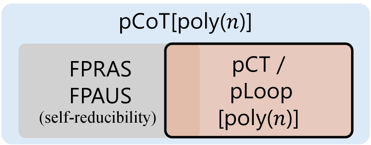
## Diagram: Set Relationship of Approximation Algorithms ### Overview The image is a diagram illustrating the relationship between different classes of approximation algorithms within the complexity class pCoT[poly(n)]. It shows two main categories: FPRAS/FPAUS and pCT/pLoop, with FPRAS/FPAUS being further described as (self-reducibility). ### Components/Axes * **Outer Box:** Light blue box labeled "pCoT[poly(n)]". This represents the overall complexity class. * **Left Box:** Light gray box labeled "FPRAS" and "FPAUS" with the descriptor "(self-reducibility)". * **Right Box:** Light orange box labeled "pCT / pLoop [poly(n)]". ### Detailed Analysis or Content Details * **pCoT[poly(n)]:** This is the overarching category, likely representing problems solvable within polynomial time using a specific type of computation. * **FPRAS/FPAUS:** These are two types of fully polynomial randomized approximation schemes/algorithms. The text "(self-reducibility)" indicates a property of these algorithms. * **pCT/pLoop [poly(n)]:** These are other types of approximation algorithms, possibly related to polynomial-time computation with specific characteristics. The "[poly(n)]" likely indicates a polynomial time complexity. ### Key Observations * The diagram shows that FPRAS/FPAUS and pCT/pLoop are distinct (but potentially overlapping) subsets within pCoT[poly(n)]. * The self-reducibility property is specifically associated with FPRAS/FPAUS. ### Interpretation The diagram illustrates a classification of approximation algorithms within a specific complexity class. It suggests that FPRAS/FPAUS and pCT/pLoop are different approaches to solving problems within pCoT[poly(n)]. The self-reducibility property highlights a specific characteristic of the FPRAS/FPAUS algorithms. The diagram implies that both FPRAS/FPAUS and pCT/pLoop are contained within pCoT[poly(n)], but it does not explicitly state whether they are mutually exclusive or if there is overlap between them.