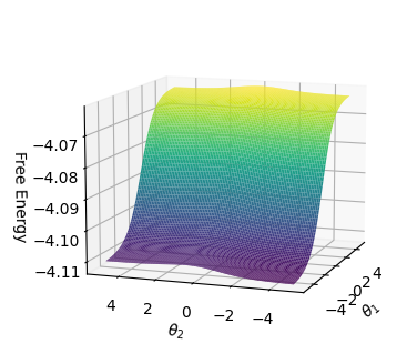
## 3D Surface Plot: Free Energy Landscape ### Overview The image displays a three-dimensional surface plot illustrating the relationship between "Free Energy" and two parameters, labeled θ₁ (theta-one) and θ₂ (theta-two). The plot visualizes a smooth, continuous surface that forms a valley or basin, indicating a region of minimum free energy. ### Components/Axes * **Vertical Axis (Z-axis):** Labeled "Free Energy". The scale is numerical, with major tick marks at -4.11, -4.10, -4.09, -4.08, and -4.07. The values are negative, indicating the energy scale. * **Horizontal Axis 1 (X-axis, front-left):** Labeled "θ₂". The scale ranges from -4 to 4, with major tick marks at -4, -2, 0, 2, and 4. * **Horizontal Axis 2 (Y-axis, front-right):** Labeled "θ₁". The scale also ranges from -4 to 4, with major tick marks at -4, -2, 0, 2, and 4. * **Color Legend:** A vertical color bar is positioned on the right side of the plot. It maps the Free Energy value to a color gradient: * **Purple/Dark Blue:** Corresponds to the lowest Free Energy values (approximately -4.11). * **Teal/Green:** Corresponds to intermediate Free Energy values (approximately -4.09 to -4.08). * **Yellow:** Corresponds to the highest Free Energy values shown (approximately -4.07). * **Grid:** A 3D wireframe grid is present on the plot's bounding box to aid in spatial orientation. ### Detailed Analysis * **Surface Topology:** The surface is bowl-shaped, with its lowest point (minimum Free Energy) located near the center of the θ₁-θ₂ plane, where both parameters are close to 0. * **Trend Verification:** * As one moves away from the origin (θ₁=0, θ₂=0) in any direction along the θ₁ or θ₂ axes, the Free Energy value increases (becomes less negative). * The slope of the surface is gentlest near the minimum and becomes steeper as the distance from the center increases. * The color gradient confirms this trend: the central region is dark purple (lowest energy), transitioning through teal and green to yellow (highest energy) at the corners of the plotted domain. * **Data Point Estimation (Approximate):** * **Minimum:** At (θ₁ ≈ 0, θ₂ ≈ 0), Free Energy ≈ -4.11. * **At Extremes:** At the corners of the plotted cube, such as (θ₁ = 4, θ₂ = 4) or (θ₁ = -4, θ₂ = -4), the Free Energy rises to approximately -4.07. * **Along Axes:** Moving along the θ₁ axis while holding θ₂=0 (or vice versa), the energy increases from ~-4.11 at the center to ~-4.08 at θ=±4. ### Key Observations 1. **Single Global Minimum:** The landscape features one clear, broad minimum basin centered at the origin. 2. **Symmetry:** The surface appears roughly symmetric with respect to both the θ₁=0 and θ₂=0 planes, suggesting the underlying function is even in both parameters. 3. **Smoothness:** The surface is smooth and continuous, with no visible discontinuities, sharp ridges, or local minima within the displayed range. 4. **Parameter Sensitivity:** The gradient (rate of change) of Free Energy appears similar with respect to changes in θ₁ and θ₂, indicating comparable sensitivity of the system to both parameters. ### Interpretation This plot represents an **energy landscape** or **cost function** common in fields like statistical mechanics, optimization, and machine learning. * **What it Demonstrates:** The system's "Free Energy" is minimized when both control parameters, θ₁ and θ₂, are set to zero. This point (0,0) represents the most stable or optimal state of the system under the modeled conditions. * **Relationship Between Elements:** The two parameters (θ₁, θ₂) are independent variables that jointly determine the system's state (Free Energy). The 3D surface maps every possible combination of these parameters to an energy value. * **Underlying Meaning:** The bowl shape implies that any deviation from the optimal parameter set (0,0) increases the system's energy, making it less stable. The smoothness suggests the system can be optimized using gradient-based methods. The symmetry might indicate that the parameters play analogous roles in the underlying physical or mathematical model. This type of visualization is crucial for understanding the stability of a solution and the behavior of an optimization algorithm navigating this landscape.