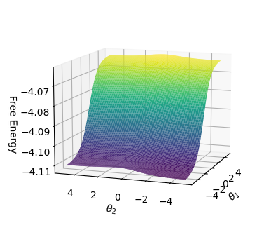
## 3D Surface Plot: Free Energy Landscape ### Overview The image depicts a 3D surface plot representing a free energy landscape as a function of two variables, θ₁ and θ₂. The surface exhibits a smooth gradient transitioning from purple (low energy) to yellow (high energy), with grid lines visible on all axes. The plot is oriented in a Cartesian coordinate system, with θ₁ and θ₂ spanning from -4 to 4 and free energy values ranging from -4.11 to -4.07. --- ### Components/Axes - **X-axis (θ₁)**: Labeled "θ₁" with a linear scale from -4 to 4. - **Y-axis (θ₂)**: Labeled "θ₂" with a linear scale from -4 to 4. - **Z-axis (Free Energy)**: Labeled "Free Energy" with a linear scale from -4.11 (minimum) to -4.07 (maximum). - **Surface**: A continuous 3D surface with a color gradient from purple (low energy) to yellow (high energy). - **Grid Lines**: Visible on all axes, providing spatial reference for the surface. --- ### Detailed Analysis - **Energy Gradient**: - The surface slopes downward from yellow (highest energy, ~-4.07) to purple (lowest energy, ~-4.11) as θ₁ and θ₂ increase. - The color transition is smooth, indicating a gradual change in energy values across the θ₁-θ₂ plane. - **Surface Shape**: - The plot forms a saddle-like structure, with the lowest energy concentrated near θ₁ = 4, θ₂ = 4 (purple region). - The highest energy is observed near θ₁ = -4, θ₂ = -4 (yellow region). - **Grid Resolution**: - Grid lines are evenly spaced, with approximately 10–12 divisions per axis, suggesting a resolution of ~0.4–0.5 units per division. --- ### Key Observations 1. **Monotonic Energy Decrease**: - Free energy decreases consistently as θ₁ and θ₂ move from negative to positive values. 2. **Color-Energy Correlation**: - Purple corresponds to the minimum energy (-4.11), while yellow corresponds to the maximum energy (-4.07). 3. **Smoothness**: - No abrupt changes or discontinuities in the surface, indicating a well-behaved energy landscape. --- ### Interpretation The plot represents a **continuous, differentiable energy landscape** where free energy decreases monotonically with increasing θ₁ and θ₂. This suggests a system (e.g., thermodynamic, mechanical, or optimization) that evolves toward lower energy states as θ₁ and θ₂ increase. The absence of local minima or maxima implies a single global minimum at θ₁ = 4, θ₂ = 4, which could represent an equilibrium or optimal state. The smooth gradient may indicate a linear or quadratic relationship between the variables and energy, though higher-resolution data would be needed to confirm the exact functional form. The visualization emphasizes the importance of θ₁ and θ₂ in determining system stability, with practical implications for parameter tuning in fields like machine learning, physics, or engineering.