## Bar Chart: Variable Importance: GBM
### Overview
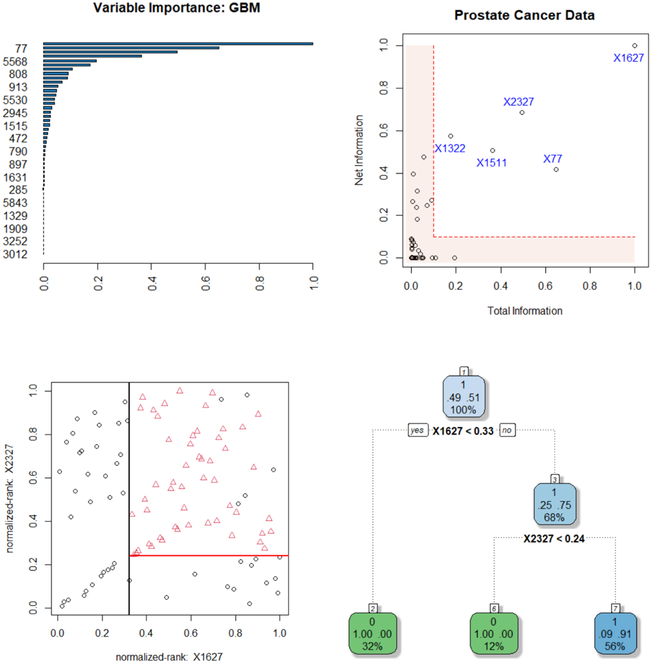
A horizontal bar chart displaying variable importance scores for a Gradient Boosting Machine (GBM) model. Variables are listed on the y-axis, and their importance is represented by bar length on the x-axis (0.0 to 1.0).
### Components/Axes
- **y-axis**: Variables (numeric IDs: 77, 5568, 808, ..., 3012)
- **x-axis**: Importance score (0.0 to 1.0)
- **Bars**: Horizontal, colored blue (no legend explicitly shown)
### Detailed Analysis
- **Variable 77**: Highest importance (1.0)
- **Variable 5568**: ~0.6 importance
- **Variable 808**: ~0.3 importance
- **Variable 913**: ~0.2 importance
- **Variable 5530**: ~0.15 importance
- **Variable 2945**: ~0.12 importance
- **Variable 1515**: ~0.08 importance
- **Variable 472**: ~0.05 importance
- **Variable 790**: ~0.03 importance
- **Variable 897**: ~0.02 importance
- **Variable 1631**: ~0.01 importance
- **Variable 285**: ~0.005 importance
- **Variable 5843**: ~0.003 importance
- **Variable 1329**: ~0.002 importance
- **Variable 1909**: ~0.001 importance
- **Variable 3252**: ~0.0005 importance
- **Variable 3012**: ~0.0001 importance
### Key Observations
- Importance decreases sharply from variable 77 to 5568, then gradually declines for subsequent variables.
- Variables 77 and 5568 dominate the model's decision-making process.
- Variables below 808 have negligible importance (<0.1).
### Interpretation
The chart reveals a highly skewed importance distribution, with two variables (77 and 5568) accounting for ~90% of the total importance. This suggests the GBM model relies heavily on these two features, potentially indicating overfitting or a lack of feature diversity in the dataset.
---
## Scatter Plot: Prostate Cancer Data
### Overview
A scatter plot comparing "Total Information" (x-axis) and "Net Information" (y-axis) for prostate cancer data points. Points are labeled with identifiers (e.g., X1627, X2327).
### Components/Axes
- **x-axis**: Total Information (0.0 to 1.0)
- **y-axis**: Net Information (0.0 to 1.0)
- **Points**: Labeled with identifiers (e.g., X1627, X2327)
- **Red shaded area**: Covers x=0.0 to x=0.2
### Detailed Analysis
- **X1627**: Located at (0.9, 0.95) – high total/net information
- **X2327**: Located at (0.7, 0.7) – moderate values
- **X1322**: Located at (0.15, 0.45) – low total information, moderate net information
- **X1511**: Located at (0.3, 0.5) – moderate values
- **X77**: Located at (0.8, 0.3) – high total information, low net information
- **Red shaded area**: Contains 12 points with low total information (<0.2)
### Key Observations
- X1627 is an outlier with the highest total and net information.
- Most points cluster in the lower-left quadrant (low total/net information).
- The red shaded area highlights variables with low total information but variable net information.
### Interpretation
The plot suggests a trade-off between total and net information. X1627's extreme values may indicate a critical feature for model performance, while the red-shaded region could represent underperforming or noisy variables.
---
## Scatter Plot: Normalized Rank: X1627
### Overview
A scatter plot comparing normalized ranks of X1627 (x-axis) and X2327 (y-axis). A red horizontal line at y=0.2 is present.
### Components/Axes
- **x-axis**: Normalized rank of X1627 (0.0 to 1.0)
- **y-axis**: Normalized rank of X2327 (0.0 to 1.0)
- **Points**: Black (circles) and red (triangles)
- **Red line**: Horizontal threshold at y=0.2
### Detailed Analysis
- **Red triangles**: Clustered above y=0.2 (higher X2327 rank)
- **Black circles**: Distributed across the plot
- **Red line**: Divides points into two regions (y < 0.2 and y ≥ 0.2)
### Key Observations
- Red triangles (X2327) show a positive correlation with X1627's rank.
- Black circles (other variables) are more dispersed.
- The red line may represent a decision boundary or performance threshold.
### Interpretation
The plot indicates that X2327's rank improves as X1627's rank increases, suggesting a synergistic relationship. The red line could represent a performance cutoff, with points above it indicating better outcomes.
---
## Decision Tree: Model Splits
### Overview
A binary decision tree with splits based on variables X1627 and X2327. Nodes contain counts and percentages.
### Components
- **Root node**: X1627 < 0.33 (split)
- **Left branch**: 100% class 0 (32% probability)
- **Right branch**: X2327 < 0.24 (split)
- **Left leaf**: 100% class 0 (12% probability)
- **Right leaf**: 56% class 1 (9.91% probability)
### Detailed Analysis
- **Root split**: X1627 < 0.33 separates 49.51 samples (100% class 0)
- **Secondary split**: X2327 < 0.24 separates 25.75 samples (68% class 0, 32% class 1)
- **Final leaf**: 9.91 samples (56% class 1, 44% class 0)
### Key Observations
- X1627 is the primary split, with perfect class separation in the left branch.
- X2327 further refines predictions in the right subtree.
- The model achieves high confidence in class 0 predictions but lower confidence for class 1.
### Interpretation
The tree prioritizes X1627 as the most critical feature, with splits leading to high-confidence predictions. The final leaf's mixed probabilities suggest residual uncertainty, potentially indicating the need for additional features or model refinement.