## Chart/Diagram Type: Audio Signal Analysis
### Overview
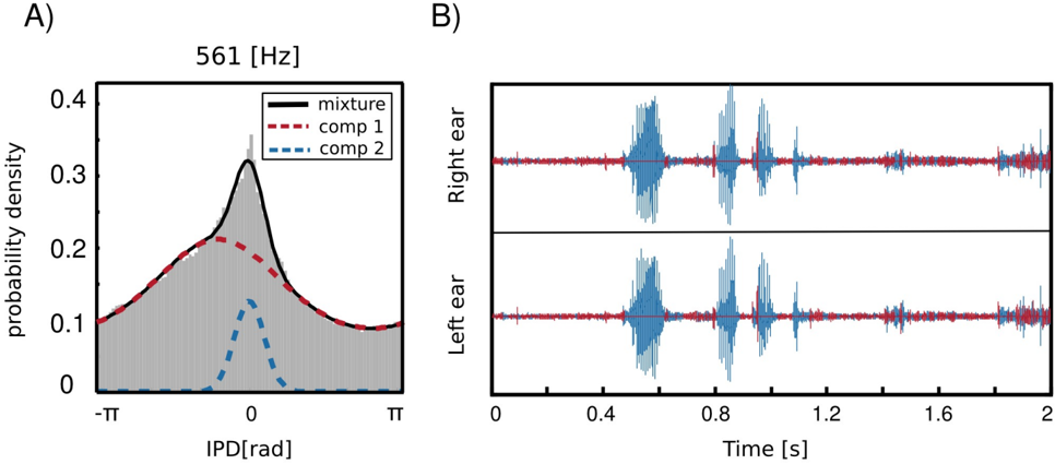
The image presents two plots analyzing audio signals. Plot A shows the probability density of the Interaural Phase Difference (IPD) for a mixture signal and its two components at 561 Hz. Plot B displays the time-domain waveforms of the audio signal recorded at the right and left ears.
### Components/Axes
**Plot A:**
* **Title:** 561 [Hz]
* **X-axis:** IPD [rad], with markers at -π, 0, and π.
* **Y-axis:** probability density, with markers at 0, 0.1, 0.2, 0.3, and 0.4.
* **Legend (top-right of Plot A):**
* Black line: mixture
* Red dashed line: comp 1
* Blue dashed line: comp 2
* **Data:** The plot shows a histogram (grey bars) representing the distribution of IPD values for the mixture. Overlaid on the histogram are curves representing the probability densities of the mixture (black), component 1 (red dashed), and component 2 (blue dashed).
**Plot B:**
* **X-axis:** Time [s], with markers at 0, 0.4, 0.8, 1.2, 1.6, and 2.
* **Y-axis:** Two traces are shown, labeled "Right ear" (top) and "Left ear" (bottom). The y-axis is not explicitly labeled with units, but it represents the amplitude of the audio signal.
* **Data:** The plot shows the audio signal waveforms for the right and left ears over a 2-second interval. The waveforms are composed of a red baseline with blue spikes.
### Detailed Analysis or ### Content Details
**Plot A (IPD Probability Density):**
* **Mixture (black line):** The mixture's IPD probability density has a peak around 0 rad, with a value of approximately 0.33. It decreases towards both -π and π, reaching a value of approximately 0.1.
* **Component 1 (red dashed line):** The IPD probability density of component 1 is broader than the mixture, with a peak around 0 rad, with a value of approximately 0.22. It decreases towards both -π and π, reaching a value of approximately 0.1.
* **Component 2 (blue dashed line):** The IPD probability density of component 2 is centered around 0 rad, with a peak value of approximately 0.1. It rapidly decreases away from 0.
**Plot B (Time-Domain Waveforms):**
* **Right Ear:** The waveform shows several bursts of activity (blue spikes) superimposed on a baseline (red). These bursts occur at approximately 0.4s, 0.8s, 1.2s, and 1.6s.
* **Left Ear:** The waveform is similar to the right ear, with bursts of activity at approximately the same times.
### Key Observations
* **Plot A:** The mixture's IPD distribution is a combination of the distributions of its two components. Component 1 has a broader distribution than component 2.
* **Plot B:** The audio signals recorded at the right and left ears are highly correlated, with bursts of activity occurring at similar times.
### Interpretation
The plots provide insights into the spatial characteristics of an audio signal. Plot A shows the distribution of IPD values, which is related to the perceived location of the sound source. The fact that the mixture's IPD distribution is centered around 0 suggests that the sound source is located directly in front of the listener. The presence of two components with different IPD distributions suggests that the sound source may be composed of multiple sources or reflections.
Plot B shows the time-domain waveforms of the audio signal recorded at the right and left ears. The high correlation between the two waveforms suggests that the sound source is relatively close to the listener. The bursts of activity in the waveforms likely correspond to distinct sound events.