\n
## Chart/Diagram Type: Auditory Signal Analysis - IPD Distribution & Waveforms
### Overview
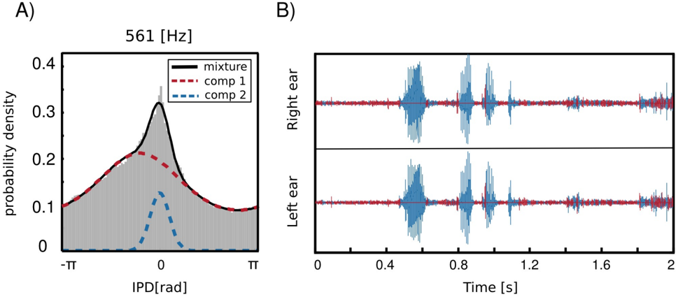
The image presents two panels (A and B) related to auditory signal processing. Panel A displays a probability density function (PDF) of the Interaural Phase Difference (IPD) for a 561 Hz tone, showing the distribution for a mixture signal and its two components. Panel B shows the waveforms of the signal in the right and left ears over time.
### Components/Axes
**Panel A:**
* **Title:** "561 [Hz]" - indicating the frequency of the analyzed tone.
* **X-axis:** "IPD[rad]" - Interaural Phase Difference in radians, ranging from approximately -π to π.
* **Y-axis:** "probability density" - ranging from 0 to 0.4.
* **Legend:**
* "mixture" - represented by a solid black line and filled grey area.
* "comp 1" - represented by a dashed red line.
* "comp 2" - represented by a dashed blue line.
**Panel B:**
* **X-axis:** "Time [s]" - Time in seconds, ranging from 0 to 2.
* **Y-axis:** No explicit label, but represents the amplitude of the signal.
* **Labels:**
* "Right ear" - above the top waveform plot.
* "Left ear" - above the bottom waveform plot.
* **Waveforms:**
* Grey waveforms representing the auditory signal.
* Red lines overlaid on the waveforms, likely representing an envelope or another processed signal.
### Detailed Analysis or Content Details
**Panel A: IPD Distribution**
* **Mixture (Black):** The IPD distribution for the mixture signal is approximately Gaussian-shaped, peaking near 0 rad. The maximum probability density is approximately 0.33. The distribution extends from approximately -π to π, with a slight asymmetry.
* **Comp 1 (Red):** The IPD distribution for component 1 is a single peak centered around approximately -0.5 rad. The maximum probability density is approximately 0.18.
* **Comp 2 (Blue):** The IPD distribution for component 2 is a single peak centered around approximately 0.5 rad. The maximum probability density is approximately 0.11.
* The combined distributions of Comp 1 and Comp 2 create the mixture distribution.
**Panel B: Waveforms**
* **Right Ear:** The waveform shows a series of peaks and troughs, indicating a periodic signal. The red line appears to follow the general envelope of the waveform, with some deviations. The waveform appears to be a complex signal with multiple components.
* **Left Ear:** The waveform is similar to the right ear, but with a phase shift. The red line again follows the envelope, but with similar deviations. The phase shift is visually apparent by the offset of the peaks and troughs compared to the right ear waveform.
### Key Observations
* The IPD distribution of the mixture signal is centered around 0 rad, suggesting that the signal is largely in-phase between the two ears.
* The two components (Comp 1 and Comp 2) have IPDs shifted to the left and right, respectively. This suggests that these components are spatially separated.
* The waveforms in the right and left ears are similar but phase-shifted, consistent with the IPD information.
* The red lines in Panel B do not appear to be a simple envelope, as they deviate from the peak amplitudes in several places.
### Interpretation
The data suggests an analysis of a sound source composed of two distinct components. The IPD distributions indicate that these components originate from different spatial locations. The mixture signal's IPD distribution reflects the combination of these two components. The waveforms in Panel B confirm the phase difference between the ears, which is the basis for spatial hearing. The red lines in Panel B could represent a processed signal, such as a smoothed version of the waveform or a different frequency component. The fact that the red line doesn't perfectly track the waveform suggests a more complex relationship than a simple envelope. This could be related to the decomposition of the signal into its components, as suggested by the IPD analysis. The analysis is likely related to sound localization or binaural hearing research.