## Diagram: Dot Product Computation Graph
### Overview
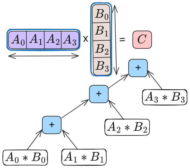
The image is a technical diagram illustrating the step-by-step computation of the dot product (scalar product) between two 4-element vectors, resulting in a single scalar value, `C`. It uses a tree-like computational graph to break down the operation into its fundamental multiplications and additions.
### Components/Axes
The diagram is composed of several distinct visual components:
1. **Input Vectors (Top Region):**
* **Vector A:** A horizontal, purple-filled rectangle containing four elements labeled `A₀`, `A₁`, `A₂`, `A₃` from left to right. A double-headed arrow beneath it indicates its span.
* **Vector B:** A vertical, beige-filled rectangle containing four elements labeled `B₀`, `B₁`, `B₂`, `B₃` from top to bottom. A double-headed arrow to its right indicates its span.
* **Operation Symbols:** A multiplication symbol (`×`) is placed between the two vectors. An equals sign (`=`) is placed to the right of Vector B.
* **Result:** A pink-filled square labeled `C` is positioned to the right of the equals sign, representing the final scalar output.
2. **Computational Graph (Main/Lower Region):**
* **Leaf Nodes (Bottom):** Four white rectangular boxes with black borders, each containing a multiplication term: `A₀ * B₀`, `A₁ * B₁`, `A₂ * B₂`, and `A₃ * B₃`. These represent the pairwise multiplications of corresponding vector elements.
* **Internal Nodes:** Three blue, rounded squares, each containing a plus sign (`+`). These represent addition operations.
* **Edges:** Black arrows connect the nodes, indicating the flow of data. The arrows converge from the multiplication leaves into the addition nodes, and from the addition nodes upward toward the final result `C`.
### Detailed Analysis
The diagram explicitly maps the mathematical formula for a dot product: `C = A₀*B₀ + A₁*B₁ + A₂*B₂ + A₃*B₃`.
**Spatial Grounding & Flow:**
The computation flows from the bottom of the diagram upward.
1. **Bottom Layer:** The four element-wise products (`A₀*B₀`, `A₁*B₁`, `A₂*B₂`, `A₃*B₃`) are computed in parallel.
2. **First Addition Layer:** The products `A₀*B₀` and `A₁*B₁` are fed into the leftmost blue `+` node. The products `A₂*B₂` and `A₃*B₃` are fed into the rightmost blue `+` node.
3. **Second Addition Layer:** The results from the two lower addition nodes are fed into the central, higher blue `+` node.
4. **Result:** The output of the central addition node is the final value `C`, as indicated by the arrow pointing to the pink `C` box at the top right.
This structure represents a balanced binary tree for summation, which is a common pattern in parallel computing for reducing a list of numbers to a single sum.
### Key Observations
* **Explicit Decomposition:** The diagram leaves no operation implicit. Every multiplication and every addition required for the dot product is visually represented as a distinct node.
* **Hierarchical Summation:** The addition is not shown as a simple chain (`((((A₀*B₀)+(A₁*B₁))+(A₂*B₂))+(A₃*B₃))`) but as a balanced tree. This suggests an emphasis on the computational structure, potentially highlighting parallelization opportunities where the two lower-level additions can occur simultaneously.
* **Color Coding:** Colors are used functionally to group related elements: purple for the first input vector, beige for the second, pink for the final output, and blue for intermediate arithmetic operations (additions).
### Interpretation
This diagram serves as a pedagogical or technical visualization of a fundamental linear algebra operation. It translates the compact mathematical notation `C = A · B` into an explicit computational procedure.
* **What it demonstrates:** It shows that the dot product is a two-stage process: first, a set of parallel multiplications, followed by a hierarchical summation. The tree structure for addition is more efficient for parallel processing than a linear chain, as it reduces the critical path length (the longest sequence of dependent operations).
* **Relationship between elements:** The input vectors `A` and `B` are the source data. The multiplication leaves are the first transformation. The addition nodes are the reduction steps that aggregate the intermediate results into the final scalar `C`.
* **Notable Anomaly/Insight:** The diagram does not show any data values, only symbolic labels. Its purpose is to illustrate the *structure* of the computation, not a specific numerical result. The clear separation of multiplication and addition stages is the key takeaway, making it a useful tool for explaining algorithm design, hardware implementation (like in a CPU's floating-point unit), or parallel computing concepts.