## Line Chart: Convergence of HMC Step
### Overview
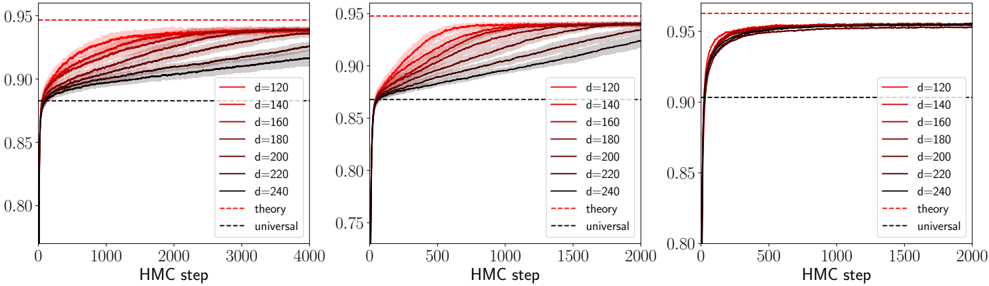
The image presents three line charts displaying the convergence of Hamiltonian Monte Carlo (HMC) steps. Each chart shows multiple lines representing different values of 'd' (dimension), along with theoretical and universal curves for comparison. The charts appear to be examining how quickly the HMC algorithm converges to a stable state as the number of steps increases.
### Components/Axes
* **X-axis:** "HMC step" - ranging from 0 to 4000 in the first chart, 0 to 2000 in the second and third chart.
* **Y-axis:** Ranges from approximately 0.75 to 0.96 in the first chart, 0.75 to 0.96 in the second chart, and 0.80 to 0.96 in the third chart. The axis is not explicitly labeled, but represents a convergence metric.
* **Legend:** Located in the top-right corner of each chart. The legend contains the following entries:
* `d=120` (Red line)
* `d=140` (Orange line)
* `d=160` (Yellow line)
* `d=180` (Green line)
* `d=200` (Blue line)
* `d=220` (Purple line)
* `d=240` (Black line)
* `theory` (Red dashed line)
* `universal` (Black dashed line)
### Detailed Analysis or Content Details
**Chart 1 (Left):**
* The lines representing different 'd' values start around 0.90 and generally increase towards a plateau around 0.95.
* The lines for `d=120` and `d=140` converge fastest, reaching the plateau relatively quickly.
* The lines for `d=220` and `d=240` converge more slowly, taking longer to reach the plateau.
* The `theory` line (red dashed) starts at approximately 0.92 and remains relatively constant around 0.95.
* The `universal` line (black dashed) starts at approximately 0.92 and remains relatively constant around 0.95.
* Approximate data points (reading from the chart):
* `d=120`: At HMC step = 0, value ≈ 0.90; At HMC step = 4000, value ≈ 0.95
* `d=240`: At HMC step = 0, value ≈ 0.89; At HMC step = 4000, value ≈ 0.94
**Chart 2 (Center):**
* Similar trend to Chart 1, but the x-axis range is shorter (0-2000).
* Convergence appears faster overall.
* Approximate data points:
* `d=120`: At HMC step = 0, value ≈ 0.89; At HMC step = 2000, value ≈ 0.95
* `d=240`: At HMC step = 0, value ≈ 0.87; At HMC step = 2000, value ≈ 0.94
**Chart 3 (Right):**
* Similar trend to Chart 1 and 2, but the x-axis range is shorter (0-2000).
* Convergence appears even faster overall.
* Approximate data points:
* `d=120`: At HMC step = 0, value ≈ 0.88; At HMC step = 2000, value ≈ 0.95
* `d=240`: At HMC step = 0, value ≈ 0.86; At HMC step = 2000, value ≈ 0.94
### Key Observations
* Convergence speed decreases as the dimension 'd' increases. Higher dimensions require more HMC steps to reach a stable state.
* The `theory` and `universal` curves provide benchmarks for convergence. The lines for different 'd' values generally approach these benchmarks.
* The three charts show the same trends, but with different x-axis ranges, suggesting that the convergence behavior is consistent across different step limits.
### Interpretation
The data suggests that the HMC algorithm's convergence rate is sensitive to the dimensionality of the problem. As the dimension 'd' increases, more HMC steps are required to achieve the same level of convergence. The `theory` and `universal` curves likely represent theoretical limits or expected convergence rates. The fact that the lines for different 'd' values approach these curves indicates that the HMC algorithm is functioning as expected. The three charts provide a visual representation of how the convergence process unfolds over time, and how the number of HMC steps affects the algorithm's performance. The consistent trends across the three charts reinforce the reliability of the observed relationship between dimensionality and convergence speed.