# Technical Document Extraction: Symbolic Aggregate Approximation (SAX) Visualization
## 1. Component Isolation
* **Header/Legend:** Located at the top-left [x: 85, y: 75]. Contains the series identifiers.
* **Main Chart Area:** Occupies the central region. Features a fluctuating time-series line, a stepped approximation line, and horizontal threshold markers.
* **Axes:**
* **X-axis:** Horizontal bottom, representing time or sequence index.
* **Y-axis:** Vertical left, representing normalized KPI values.
* **Right-side Labels:** Vertical right, representing the symbolic alphabet mapping.
---
## 2. Legend and Labels
* **Legend [Top-Left]:**
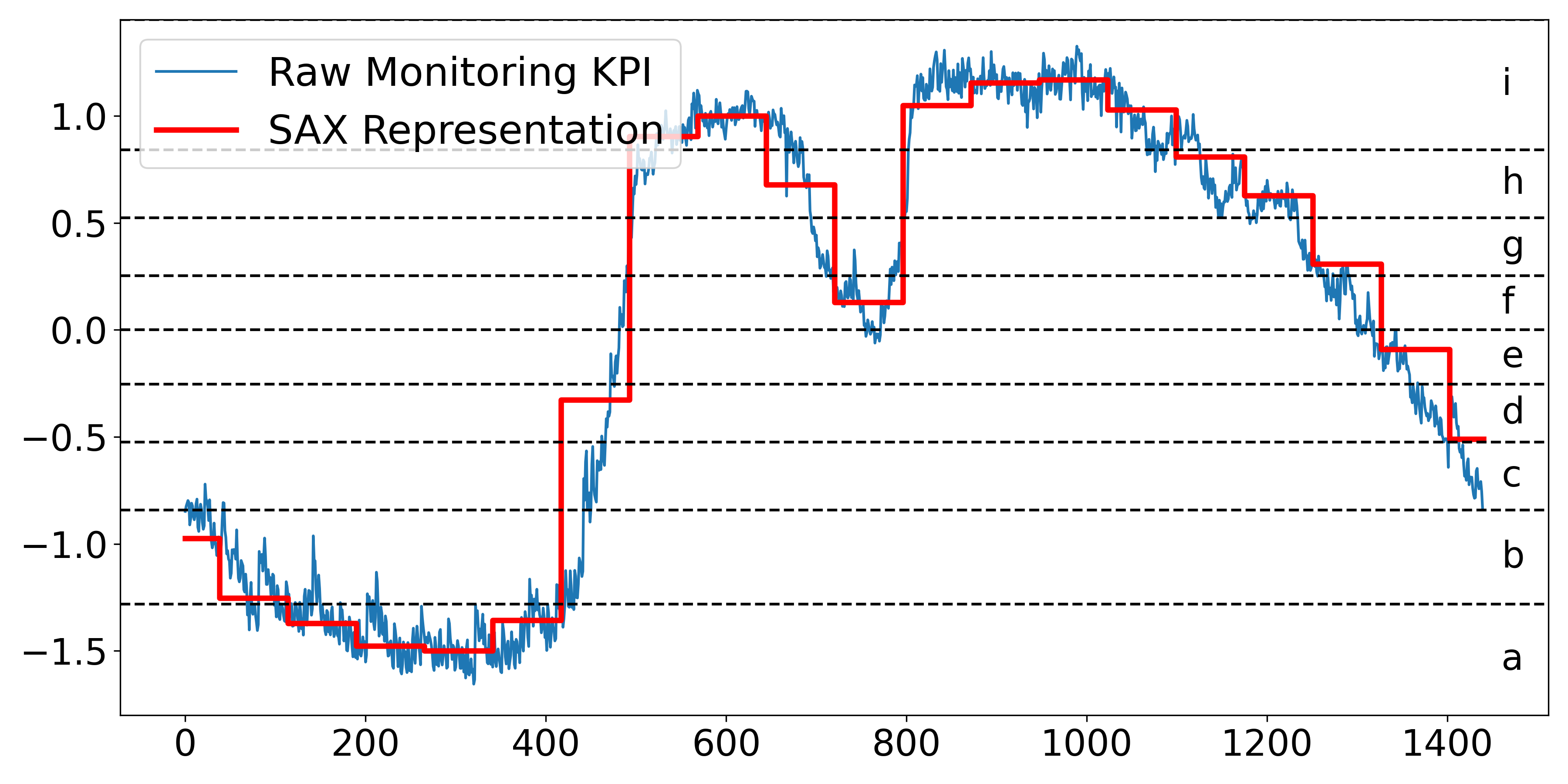
* **Blue Thin Line:** "Raw Monitoring KPI"
* **Red Thick Stepped Line:** "SAX Representation"
* **Y-Axis Markers (Left):** -1.5, -1.0, -0.5, 0.0, 0.5, 1.0
* **X-Axis Markers (Bottom):** 0, 200, 400, 600, 800, 1000, 1200, 1400
* **Symbolic Alphabet (Right):**
* The space between horizontal dashed lines is labeled with lowercase letters **a** through **i** (bottom to top).
* **i**: > ~0.85
* **h**: ~0.55 to ~0.85
* **g**: ~0.25 to ~0.55
* **f**: ~0.0 to ~0.25
* **e**: ~-0.25 to ~0.0
* **d**: ~-0.5 to ~-0.25
* **c**: ~-0.85 to ~-0.5
* **b**: ~-1.3 to ~-0.85
* **a**: < ~-1.3
---
## 3. Data Series Analysis
### Series 1: Raw Monitoring KPI (Blue Line)
* **Trend:** This is a high-frequency, noisy time-series signal.
* **Visual Flow:**
1. Starts at approx -0.9, trends downward with volatility to a trough of approx -1.6 around index 300.
2. Sharp upward climb from index 400 to 550, reaching a peak of approx 1.1.
3. Brief dip to 0.0 at index 750.
4. Second peak reaching approx 1.3 between index 800 and 1000.
5. Gradual, volatile descent from index 1000 to the end of the chart, finishing near -0.8.
### Series 2: SAX Representation (Red Stepped Line)
* **Trend:** This is a Piecewise Aggregate Approximation (PAA) converted into discrete symbols. It follows the mean of the blue line within specific time windows.
* **Visual Flow:**
* **Index 0-400:** Stays in the lower regions, stepping through levels corresponding to symbols **c, b,** and **a**.
* **Index 400-500:** A sharp vertical jump from level **b** to level **h**.
* **Index 550-700:** Plateaus at level **i**, then drops to level **h**.
* **Index 700-800:** Drops to level **f**.
* **Index 800-1050:** Sustained plateau at level **i**.
* **Index 1050-1450:** Sequential downward steps through levels **h, g, f, e,** and finally **d**.
---
## 4. Data Table Reconstruction (Approximated)
The following table represents the SAX transformation logic visible in the chart, mapping the Red Line's position to the symbolic alphabet.
| Time Window (Approx Index) | SAX Level (Red Line Value) | Symbolic Label |
| :--- | :--- | :--- |
| 0 - 50 | ~ -1.0 | c |
| 50 - 120 | ~ -1.25 | b |
| 120 - 180 | ~ -1.35 | a |
| 180 - 350 | ~ -1.5 | a |
| 350 - 420 | ~ -1.35 | a |
| 420 - 480 | ~ -0.3 | d |
| 480 - 550 | ~ 0.9 | i |
| 550 - 650 | ~ 1.0 | i |
| 650 - 720 | ~ 0.7 | h |
| 720 - 800 | ~ 0.15 | f |
| 800 - 1050 | ~ 1.1 | i |
| 1050 - 1120 | ~ 1.0 | i |
| 1120 - 1180 | ~ 0.8 | h |
| 1180 - 1250 | ~ 0.6 | h |
| 1250 - 1320 | ~ 0.3 | g |
| 1320 - 1400 | ~ -0.1 | e |
| 1400 - 1450 | ~ -0.5 | d |
---
## 5. Technical Summary
The image demonstrates the **Symbolic Aggregate Approximation (SAX)** algorithm applied to a noisy KPI signal. The process involves:
1. **Normalization:** The Y-axis indicates the signal is likely Z-normalized.
2. **PAA (Piecewise Aggregate Approximation):** The signal is divided into equal-sized time windows, and the mean of each window is calculated (the horizontal segments of the red line).
3. **Discretization:** The PAA values are mapped to discrete symbols (**a-i**) based on predefined breakpoints (the horizontal dashed lines). This transforms a continuous time-series into a string of characters for efficient pattern matching and storage.