## Diagram: Deductive vs. Inductive Learning ### Overview The image presents two diagrams illustrating deductive and inductive learning approaches. Diagram (A) depicts the deductive approach, where fixed rules are used to learn content. Diagram (B) illustrates the inductive approach, where a fixed input is used to learn structure. Both diagrams show a flow of information between components, with feedback loops indicated by "Gradient (∇)". ### Components/Axes **Diagram (A) - Deductive:** * **Title:** (A) Deductive * **Subtitle:** Fixed Rules, Learn Content * **Components:** * Proposer NN (Learns State) - Located on the left, in a blue box. * Differentiable Modal Logic - Located in the center, in a blue box. * Loss (Ltask + Lcontra) - Located on the right, in a purple box. * Relation (Fixed R/Learned Aθ) - Located at the top-right, in an orange box. * **Flow:** * Proposer NN -> Differentiable Modal Logic -> Loss -> Relation * Gradient (∇) - An orange arrow from Loss back to Proposer NN, and from Relation back to Differentiable Modal Logic. **Diagram (B) - Inductive:** * **Title:** (B) Inductive * **Subtitle:** Fixed Input, Learn Structure * **Components:** * Context Enc. (Fixed Input) - Located on the left, in a gray box. * Differentiable Modal Logic - Located in the center, in a blue box. * Loss (Ltask + Lcontra) - Located on the right, in a purple box. * Relation NN (Learns Aθ) - Located at the top-right, in an orange box. * **Flow:** * Context Enc. -> Differentiable Modal Logic -> Loss -> Relation NN * Gradient (∇) - An orange arrow from Loss to Context Enc., and from Relation NN back to Differentiable Modal Logic. ### Detailed Analysis or Content Details **Diagram (A) - Deductive:** * The Proposer NN learns the state and feeds it into the Differentiable Modal Logic. * The Differentiable Modal Logic processes the state and calculates a loss. * The Loss is calculated as Ltask + Lcontra. * The Relation component has fixed rules (R) but learns Aθ. * The Gradient (∇) provides feedback from the Loss to the Proposer NN and from Relation to Differentiable Modal Logic. **Diagram (B) - Inductive:** * The Context Enc. takes a fixed input and feeds it into the Differentiable Modal Logic. * The Differentiable Modal Logic processes the input and calculates a loss. * The Loss is calculated as Ltask + Lcontra. * The Relation NN learns Aθ. * The Gradient (∇) provides feedback from the Loss to the Context Enc. and from Relation NN to Differentiable Modal Logic. ### Key Observations * Both diagrams share similar components: Differentiable Modal Logic and Loss. * The main difference lies in the input and the learning objective. Deductive learning starts with fixed rules and learns content, while inductive learning starts with a fixed input and learns structure. * The feedback loop (Gradient (∇)) is present in both diagrams, indicating an iterative learning process. * The Loss function is the same in both approaches (Ltask + Lcontra). ### Interpretation The diagrams illustrate two fundamental approaches to machine learning: deductive and inductive. Deductive learning is akin to applying known rules to new data, while inductive learning involves inferring rules from data. The diagrams highlight the flow of information and the role of feedback in both approaches. The use of "Differentiable Modal Logic" suggests a specific type of learning model is being employed. The "Loss" component represents the error signal that drives the learning process. The "Gradient (∇)" indicates the direction and magnitude of adjustments made to the model's parameters during training. The diagrams suggest that both approaches involve iterative refinement of the model based on the feedback from the loss function.

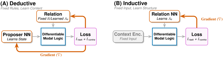
## Diagram: Comparison of Deductive and Inductive Learning Architectures ### Overview The image displays two schematic diagrams, labeled (A) and (B), illustrating two distinct machine learning paradigms: **Deductive** and **Inductive**. Both architectures utilize a shared core component, "Differentiable Modal Logic," and a "Loss" function, but they differ in their input sources, what is being learned, and the feedback pathways. ### Components/Axes The diagrams use a consistent color-coding scheme to denote the function of each block: * **Orange Boxes:** Learnable components (Proposer NN, Relation, Relation NN). * **Blue Boxes:** Core processing unit (Differentiable Modal Logic). * **Pink Boxes:** Optimization/Output component (Loss). * **Grey Box:** Fixed/Static input (Context Enc.). * **Arrows:** Indicate data flow (grey) and gradient feedback loops (orange). ### Detailed Analysis #### (A) Deductive (Fixed Rules, Learn Content) * **Flow:** 1. **Proposer NN** (labeled "Learns State") feeds into **Differentiable Modal Logic**. 2. **Relation** (labeled "Fixed R/Learned $A_\theta$") feeds into **Differentiable Modal Logic**. 3. **Differentiable Modal Logic** feeds into **Loss** (labeled "$L_{task} + L_{contra}$"). * **Feedback:** The **Loss** module propagates a "Gradient ($\nabla$)" back to both the **Relation** module and the **Proposer NN**. * **Logic:** This architecture is designed to learn the *content* (state) while operating under fixed rules. #### (B) Inductive (Fixed Input, Learn Structure) * **Flow:** 1. **Context Enc.** (labeled "Fixed Input") feeds into **Differentiable Modal Logic**. 2. **Relation NN** (labeled "Learns $A_\theta$") feeds into **Differentiable Modal Logic**. 3. **Differentiable Modal Logic** feeds into **Loss** (labeled "$L_{task} + L_{contra}$"). * **Feedback:** The **Loss** module propagates a "Gradient ($\nabla$)" back to the **Relation NN**. * **Logic:** This architecture is designed to learn the *structure* (the relations) while operating on a fixed input. ### Key Observations * **Shared Core:** Both diagrams utilize the exact same "Differentiable Modal Logic" and "Loss" modules, suggesting these are the invariant components of the system. * **Feedback Asymmetry:** Diagram (A) features a dual-feedback loop (updating both the Proposer and the Relation), whereas Diagram (B) features a single-feedback loop (updating only the Relation NN). * **Input/State Distinction:** In (A), the system learns the "State" (Proposer NN). In (B), the system receives a "Fixed Input" (Context Enc.), shifting the learning burden entirely to the "Relation NN." * **Notation:** Both diagrams use the notation $A_\theta$ to represent the learned parameters of the relation, and $L_{task} + L_{contra}$ to represent the combined loss function (likely a combination of task-specific loss and contrastive loss). ### Interpretation This diagram illustrates the fundamental tension between deductive and inductive reasoning within the context of differentiable logic systems. * **Deductive (Top-Down):** The system starts with a set of "Fixed Rules" (the logic framework) and attempts to learn the "Content" (the state of the world). It is essentially trying to map observed states into a pre-defined logical structure. The feedback loop to the "Proposer NN" indicates that the system is actively refining its understanding of the state to better fit the fixed rules. * **Inductive (Bottom-Up):** The system starts with a "Fixed Input" (the raw data or context) and attempts to "Learn Structure." It is trying to infer the logical rules (the relations) that govern the data. The feedback loop only updates the "Relation NN," suggesting the system is refining its internal model of the logic itself to better explain the fixed input. In essence, these diagrams demonstrate how the same "Differentiable Modal Logic" engine can be repurposed: either to find the best state for a given rule (Deductive) or to find the best rule for a given state (Inductive).

## Diagram: Deductive vs. Inductive Neural Network Architectures ### Overview The image compares two neural network architectures: **Deductive** (A) and **Inductive** (B). Both involve a **Differentiable Modal Logic** component and a **Loss** function, but differ in their structural design principles and learning objectives. ### Components/Axes #### (A) Deductive - **Title**: "Deductive" - **Subtitle**: "Fixed Rules, Learn Content" - **Components**: 1. **Proposer NN**: "Learns State" (orange box with bidirectional arrow). 2. **Relation**: "Fixed R/Learned Aθ" (orange box with unidirectional arrow to Differentiable Modal Logic). 3. **Differentiable Modal Logic**: Central blue box with gradient (∇) annotation. 4. **Loss**: "L_task + L_contra" (purple box). - **Flow**: - Proposer NN → Relation → Differentiable Modal Logic → Loss. - Gradient (∇) flows from Loss back to Proposer NN. #### (B) Inductive - **Title**: "Inductive" - **Subtitle**: "Fixed Input, Learn Structure" - **Components**: 1. **Context Enc.**: "Fixed Input" (gray box with unidirectional arrow). 2. **Relation NN**: "Learns Aθ" (orange box with unidirectional arrow to Differentiable Modal Logic). 3. **Differentiable Modal Logic**: Central blue box (shared with Deductive). 4. **Loss**: "L_task + L_contra" (purple box). - **Flow**: - Context Enc. → Relation NN → Differentiable Modal Logic → Loss. - Gradient (∇) flows from Loss back to Relation NN. ### Detailed Analysis - **Deductive Architecture**: - **Proposer NN** learns the system state, suggesting dynamic adaptation. - **Relation** combines fixed rules (R) with learned parameters (Aθ), indicating hybrid reasoning. - Gradient (∇) propagates through the entire loop, enabling end-to-end training. - **Inductive Architecture**: - **Context Enc.** processes fixed input data, emphasizing structured input handling. - **Relation NN** learns parameters (Aθ) directly, focusing on structural adaptation. - Gradient (∇) is localized to the Relation NN and Loss, limiting backpropagation scope. ### Key Observations 1. **Shared Elements**: - Both architectures use **Differentiable Modal Logic** as a core component. - Loss function combines task-specific (L_task) and contrastive (L_contra) objectives. 2. **Divergent Designs**: - **Deductive** prioritizes learning content (state) while retaining fixed rules. - **Inductive** focuses on learning structure (Aθ) from fixed inputs. 3. **Gradient Flow**: - Deductive uses a closed-loop gradient (∇) for holistic optimization. - Inductive restricts gradients to the Relation NN and Loss, simplifying training. ### Interpretation The diagram illustrates a trade-off between **rule-based reasoning** (Deductive) and **data-driven adaptation** (Inductive). The Deductive approach leverages fixed rules for stability while learning state-specific content, whereas the Inductive method optimizes structural parameters (Aθ) to generalize from fixed inputs. The shared use of Differentiable Modal Logic suggests a unified framework for integrating symbolic reasoning with neural learning. The gradient annotations highlight differences in optimization strategies, with Deductive favoring global updates and Inductive focusing on localized parameter tuning.