## Diagram: RG Transformation Process
### Overview
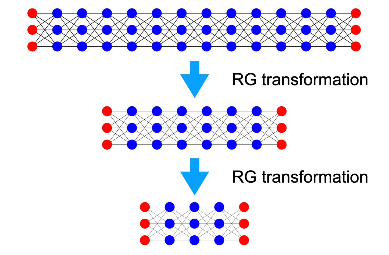
The image is a technical diagram illustrating a three-stage process labeled "RG transformation." It depicts the sequential simplification of a network structure, likely representing a renormalization group transformation in physics or network theory. The diagram flows vertically from top to bottom, with each stage showing a reduced version of the previous network.
### Components/Axes
* **Primary Elements:** Three network diagrams arranged vertically.
* **Connectors:** Two large, light blue downward-pointing arrows connect the stages.
* **Text Labels:** The phrase "RG transformation" appears in black, sans-serif font to the right of each blue arrow.
* **Network Components:**
* **Nodes:** Represented by circles. Two colors are used:
* **Red:** Located at the left and right ends of each network.
* **Blue:** Located in the central columns of each network.
* **Connections:** Thin black lines connect nodes between adjacent columns in a dense, crisscross pattern.
### Detailed Analysis
The diagram shows a clear, stepwise reduction in network complexity.
**Stage 1 (Top Network):**
* **Structure:** A rectangular grid of nodes.
* **Dimensions:** 3 rows by 15 columns.
* **Node Distribution:**
* Columns 1 and 15: 3 red nodes each.
* Columns 2 through 14: 3 blue nodes each.
* **Connections:** Each node in a column is connected to all nodes in the immediately adjacent columns to its left and right, creating a fully connected bipartite graph between neighboring layers.
**First Transformation:**
* A blue arrow points from the top network to the middle network.
* The label "RG transformation" is positioned to the right of this arrow.
**Stage 2 (Middle Network):**
* **Structure:** A smaller rectangular grid.
* **Dimensions:** 3 rows by 9 columns.
* **Node Distribution:**
* Columns 1 and 9: 3 red nodes each.
* Columns 2 through 8: 3 blue nodes each.
* **Connections:** The connection pattern is identical to Stage 1 (fully connected between adjacent columns), but applied to the smaller grid.
**Second Transformation:**
* A second blue arrow points from the middle network to the bottom network.
* The label "RG transformation" is again positioned to the right of this arrow.
**Stage 3 (Bottom Network):**
* **Structure:** The smallest rectangular grid.
* **Dimensions:** 3 rows by 5 columns.
* **Node Distribution:**
* Columns 1 and 5: 3 red nodes each.
* Columns 2 through 4: 3 blue nodes each.
* **Connections:** The same fully connected pattern between adjacent columns is maintained.
### Key Observations
1. **Consistent Structure:** The fundamental architecture—a 3-row grid with red nodes at the ends and blue nodes in the center—is preserved through all transformations.
2. **Systematic Reduction:** The number of columns decreases in a specific pattern: 15 → 9 → 5. This suggests a rule-based coarse-graining or decimation process.
3. **Preserved Connectivity:** While the network size shrinks, the local connectivity rule (each node connects to all nodes in neighboring columns) remains constant.
4. **Visual Metaphor:** The red "end" nodes may represent fixed boundary conditions or external degrees of freedom that are retained, while the internal blue nodes are subject to the transformation.
### Interpretation
This diagram visually explains the core concept of a Renormalization Group (RG) transformation applied to a lattice or network model. The process demonstrates **coarse-graining**: systematically removing degrees of freedom (the internal blue nodes) to create a simpler, effective description of the system at a larger scale.
* **What it suggests:** The transformation maps a detailed, microscopic model (Stage 1) to progressively simpler, macroscopic models (Stages 2 & 3) while attempting to preserve essential large-scale properties or behaviors. The consistent red endpoints imply that boundary conditions are held fixed during this scaling process.
* **How elements relate:** The blue arrows are the active process ("RG transformation") that acts upon the static network structures. The output of one transformation becomes the input for the next, illustrating an iterative scaling procedure.
* **Notable pattern:** The column count reduction (15→9→5) is not a simple halving. This implies a specific decimation scheme, possibly where blocks of a certain size (e.g., 3 sites) are replaced by a single effective site, which is a common RG technique. The diagram abstracts the mathematical details, focusing on the conceptual outcome: a smaller, structurally similar system.
**Language Note:** All text in the image is in English.