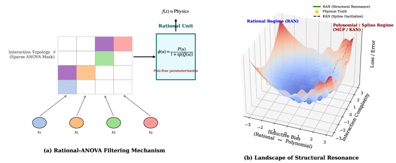
# Technical Document Extraction: Rational-ANOVA and Structural Resonance This document provides a detailed technical extraction of the provided image, which consists of two primary components: a schematic diagram of a filtering mechanism and a 3D visualization of a loss landscape. --- ## Component (a): Rational-ANOVA Filtering Mechanism This diagram illustrates the architectural flow of a data processing unit designed to approximate physical laws. ### 1. Input Layer * **Components:** Four circular nodes labeled $x_1, x_2, x_3, x_4$. * **Visual Mapping:** Each node is color-coded: * $x_1$: Light Blue * $x_2$: Orange * $x_3$: Green * $x_4$: Red/Pink * **Flow:** Arrows point from these input nodes toward a grid structure. ### 2. Interaction Topology $S$ (Sparse ANOVA Mask) * **Structure:** A $4 \times 4$ grid representing a sparse mask. * **Data Mapping:** Specific cells in the grid are colored to match the input nodes, indicating active interactions: * **Row 1:** Column 3 (Purple), Column 4 (Red/Pink) * **Row 2:** Column 3 (Green) * **Row 3:** Column 1 (Purple), Column 2 (Orange) * **Row 4:** Column 1 (Light Blue) * **Function:** This grid acts as a filter for the input variables before they enter the processing unit. ### 3. Rational Unit * **Header Text:** $f(x) \approx \text{Physics}$ * **Title:** **Rational Unit** (displayed in teal) * **Mathematical Formula:** $$\phi(u) = \frac{P(u)}{1 + \text{sp}(Q(u))}$$ * **Subtext:** "Pole-free parameterization" (displayed in red). * **Flow:** An arrow indicates the output of the Sparse ANOVA Mask serves as the input $u$ for this rational function. --- ## Component (b): Landscape of Structural Resonance This is a 3D surface plot illustrating the optimization landscape of different modeling regimes. ### 1. Axis Definitions * **X-Axis (Horizontal/Depth):** **Inductive Bias (Rational $\leftrightarrow$ Polynomial)**. Scale ranges from $-3$ to $3$. * **Y-Axis (Horizontal/Width):** **Interaction Complexity**. Scale ranges from $-3$ to $3$. * **Z-Axis (Vertical):** **Loss / Error**. ### 2. Legend and Key Markers * **Location:** Top right $[x \approx 0.8, y \approx 0.9]$ * **Green Solid Line:** RAN (Structural Resonance) * **Yellow Star:** Physical Truth * **Black Dashed Line:** KAN (Spline Oscillation) ### 3. Surface Analysis and Trends * **Overall Topology:** The surface is a complex "bowl" with multiple local minima and ripples. It is colored with a gradient where blue represents lower loss/error and red represents higher loss/error. * **Rational Regime (RAN):** * **Location:** Labeled at the top left peak area. * **Trend:** The text "Rational Regime (RAN)" points toward a deep, stable-looking valley in the blue region. * **Polynomial / Spline Regime (MLP / KAN):** * **Location:** Labeled at the top right. * **Trend:** This region is characterized by high-frequency "ripples" or oscillations on the surface. * **Visual Check:** A grey/black dashed line (representing KAN) is seen traversing these oscillatory ridges, indicating "Spline Oscillation" which leads to higher or more unstable error. * **Structural Resonance:** The "Physical Truth" (Yellow Star) is positioned at the absolute global minimum of the blue valley, coinciding with the "Rational Regime." --- ## Summary of Technical Findings | Feature | Description | | :--- | :--- | | **Primary Objective** | Approximating physics $f(x)$ using rational functions. | | **Mechanism** | Uses a Sparse ANOVA Mask to define interaction topology $S$ between inputs $x_n$. | | **Mathematical Innovation** | A pole-free rational parameterization $\phi(u)$ to prevent numerical instability. | | **Comparative Performance** | The "Rational Regime" (RAN) aligns with the "Physical Truth" at the global minimum of the loss landscape, whereas "Spline Regimes" (KAN/MLP) suffer from oscillations and higher error. |