## Scatter Plot: Correlation between $f_c$ and $f_{coh}$
### Overview
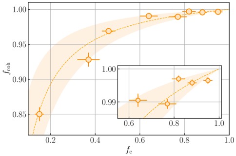
The image displays a scatter plot illustrating the relationship between two variables, $f_c$ (plotted on the x-axis) and $f_{coh}$ (plotted on the y-axis). The plot includes a main view and an inset view (located in the bottom-right quadrant) that provides a zoomed-in perspective of the high-value data points. The data is represented by orange circles with cross-hair error bars, a dashed orange trend line, and a shaded orange region representing the uncertainty or confidence interval.
### Components/Axes
**Main Plot:**
* **X-axis:** Labeled "$f_c$". The scale ranges from 0.2 to 1.0, with major grid lines at 0.2, 0.4, 0.6, 0.8, and 1.0.
* **Y-axis:** Labeled "$f_{coh}$". The scale ranges from 0.85 to 1.00, with major grid lines at 0.85, 0.90, 0.95, and 1.00.
* **Data Series:** Orange circles with horizontal and vertical error bars.
* **Trend/Uncertainty:** A dashed orange line follows the trend of the data, surrounded by a light orange shaded region representing the uncertainty interval.
**Inset Plot (Bottom-Right):**
* **Location:** Positioned in the bottom-right quadrant of the main plot.
* **X-axis:** Scale ranges from 0.6 to 1.0.
* **Y-axis:** Scale ranges from 0.99 to 1.00.
* **Content:** A zoomed-in view of the data points where $f_c > 0.6$ and $f_{coh} > 0.99$.
### Detailed Analysis
**Trend Verification:**
The data exhibits a positive, non-linear correlation. As $f_c$ increases, $f_{coh}$ increases. The curve is concave down, indicating that the rate of increase in $f_{coh}$ diminishes as $f_c$ approaches 1.0. The shaded uncertainty region is widest at the lower end of the x-axis (near $f_c = 0.2$) and narrows significantly as $f_c$ approaches 1.0, suggesting higher precision or lower variance at higher values of $f_c$.
**Data Points (Approximate Coordinates):**
| Plot | Point | $f_c$ | $f_{coh}$ |
| :--- | :--- | :--- | :--- |
| Main | 1 | $\approx 0.15$ | $\approx 0.85$ |
| Main | 2 | $\approx 0.38$ | $\approx 0.93$ |
| Main | 3 | $\approx 0.48$ | $\approx 0.97$ |
| Main | 4 | $\approx 0.62$ | $\approx 0.99$ |
| Main | 5 | $\approx 0.77$ | $\approx 0.99$ |
| Main | 6 | $\approx 0.85$ | $\approx 0.995$ |
| Main | 7 | $\approx 0.90$ | $\approx 0.995$ |
| Main | 8 | $\approx 0.96$ | $\approx 0.997$ |
| Inset | Leftmost | $\approx 0.65$ | $\approx 0.990$ |
| Inset | Bottom-middle | $\approx 0.78$ | $\approx 0.989$ |
| Inset | Top-middle | $\approx 0.83$ | $\approx 0.991$ |
| Inset | Rightmost | $\approx 0.95$ | $\approx 0.990$ |
### Key Observations
* **Asymptotic Behavior:** The trend line appears to be asymptotic to $f_{coh} = 1.0$.
* **Uncertainty Reduction:** The shaded region narrows as $f_c$ increases, indicating that the model becomes more confident or the data becomes more stable as the system approaches the maximum $f_c$ value.
* **Inset Utility:** The inset is essential because the main plot compresses the data points at the high end of the scale, making it impossible to distinguish the variance in $f_{coh}$ values between 0.99 and 1.00 without the zoom.
### Interpretation
The data demonstrates a "diminishing returns" relationship between the control parameter ($f_c$) and the coherence metric ($f_{coh}$). In many physical or engineering systems, this suggests that while increasing $f_c$ initially yields significant gains in coherence, the system eventually reaches a saturation point where further increases in $f_c$ yield negligible improvements in $f_{coh}$. The inset plot reveals that even at high $f_c$ values, there is still slight variance in the coherence, suggesting that the system does not reach a perfectly stable state of 1.0, or that measurement noise remains present even at high operating points.