# Technical Document Extraction: Decision Tree Partitioning and Node Analysis
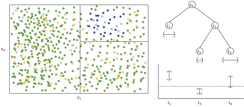
This image illustrates the relationship between a 2D feature space partition, a corresponding decision tree structure, and a statistical representation of the leaf nodes.
## 1. Component Isolation
The image is divided into three primary functional regions:
* **Left Region (Feature Space):** A 2D scatter plot showing data points and rectangular partitions.
* **Top-Right Region (Decision Tree):** A hierarchical tree diagram representing the logic used to create the partitions.
* **Bottom-Right Region (Node Statistics):** A chart showing intervals or error bars associated with the terminal leaf nodes.
---
## 2. Feature Space Analysis (Left Region)
This is a 2D coordinate system representing a feature space defined by two variables.
* **Axis Labels:**
* **X-axis:** $x_1$ (horizontal)
* **Y-axis:** $x_2$ (vertical)
* **Data Points:** The space is populated with numerous circular data points.
* **Green Points:** The majority class/type, distributed throughout the space.
* **Yellow Points:** Sparsely distributed throughout the space.
* **Blue Points:** Concentrated specifically in the top-right quadrant of the right-hand partition.
* **Transparency:** Some points appear semi-transparent, possibly indicating density or a third dimension/weight.
* **Partitions:** The space is divided by black boundary lines:
1. A primary vertical split at a specific value of $x_1$.
2. In the right-hand section ($x_1 > \text{split value}$), a horizontal split at a specific value of $x_2$.
* **Spatial Logic:**
* **Left Partition:** Contains mostly green and yellow points.
* **Top-Right Partition:** Contains a high concentration of blue points.
* **Bottom-Right Partition:** Contains mostly green and yellow points.
---
## 3. Decision Tree Diagram (Top-Right Region)
This diagram maps the recursive splitting of the feature space.
* **Nodes:** Represented by circles containing labels.
* **Root Node ($t_0$):** The starting point of the tree.
* **Internal Node ($t_2$):** A decision point following the first split.
* **Leaf Nodes ($t_1, t_3, t_4$):** Terminal nodes representing the final partitioned regions.
* **Flow/Structure:**
* $t_0$ splits into $t_1$ (left branch) and $t_2$ (right branch).
* $t_2$ splits into $t_3$ (left branch) and $t_4$ (right branch).
* **Mapping to Feature Space:**
* **$t_1$** corresponds to the large rectangular region on the left of the $x_1$ split.
* **$t_3$** corresponds to the bottom-right rectangular region.
* **$t_4$** corresponds to the top-right rectangular region (where the blue points are clustered).
* **Symbols:** Beneath each leaf node ($t_1, t_3, t_4$) is a horizontal bracket symbol indicating a range or interval associated with that node.
---
## 4. Node Statistics Chart (Bottom-Right Region)
This chart visualizes data properties for each terminal leaf node.
* **X-axis Labels:** $t_1, t_3, t_4$ (corresponding to the leaf nodes of the tree).
* **Y-axis:** Unlabeled vertical axis representing a value or magnitude.
* **Components:**
* **Dashed Horizontal Line:** Represents a baseline or threshold value across all nodes.
* **Vertical Intervals (Error Bars/Ranges):**
* **$t_1$:** A vertical interval positioned significantly **above** the dashed baseline.
* **$t_3$:** A vertical interval positioned **below** the dashed baseline.
* **$t_4$:** A vertical interval that **straddles** the dashed baseline (mostly above it).
---
## 5. Summary of Logic and Trends
1. **Partitioning Trend:** The data is first split on $x_1$ (creating node $t_1$ and $t_2$). The right-hand side ($t_2$) is then further refined by a split on $x_2$ (creating nodes $t_3$ and $t_4$).
2. **Data Correlation:** The concentration of blue points in the top-right of the feature space is captured by leaf node $t_4$.
3. **Statistical Outcome:** The chart in the bottom right indicates that the data in region $t_1$ has a higher mean/value than the baseline, region $t_3$ has a lower value, and region $t_4$ is centered near or slightly above the baseline.