## Line Chart: Per-Period Regret of Different Agents Over Time
### Overview
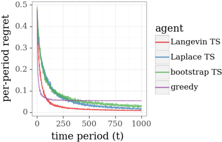
The image is a line chart comparing the performance of four different algorithms (agents) over 1000 time periods. The performance metric is "per-period regret," where a lower value indicates better performance. All agents show a decreasing trend in regret over time, but they converge to different final values and exhibit different rates of descent.
### Components/Axes
* **Chart Type:** Line chart with multiple series.
* **X-Axis:** Labeled **"time period (t)"**. The scale runs from 0 to 1000, with major tick marks at 0, 250, 500, 750, and 1000.
* **Y-Axis:** Labeled **"per-period regret"**. The scale runs from 0 to 0.5, with major tick marks at 0, 0.1, 0.2, 0.3, 0.4, and 0.5.
* **Legend:** Positioned in the **center-right** of the chart area. It is titled **"agent"** and lists four entries, each associated with a specific color:
* **Langevin TS** (Red line)
* **Laplace TS** (Blue line)
* **bootstrap TS** (Green line)
* **greedy** (Purple line)
### Detailed Analysis
The chart plots the regret value for each agent across 1000 time periods. The general trend for all agents is a sharp initial decrease followed by a gradual leveling off.
1. **Langevin TS (Red Line):**
* **Trend:** Starts at the highest point (≈0.48 at t=0), experiences the steepest initial decline, and converges to the lowest final value.
* **Data Points (Approximate):**
* t=0: ~0.48
* t=250: ~0.05
* t=500: ~0.02
* t=750: ~0.01
* t=1000: ~0.005 (approaching zero)
2. **Laplace TS (Blue Line):**
* **Trend:** Follows a very similar trajectory to Langevin TS but remains consistently slightly higher after the initial drop. Its descent is smooth.
* **Data Points (Approximate):**
* t=0: ~0.45
* t=250: ~0.08
* t=500: ~0.04
* t=750: ~0.03
* t=1000: ~0.02
3. **bootstrap TS (Green Line):**
* **Trend:** Starts similarly high but exhibits more volatility (visible "jitter" in the line) during its descent compared to the red and blue lines. It converges to a value between Langevin/Laplace TS and the greedy agent.
* **Data Points (Approximate):**
* t=0: ~0.42
* t=250: ~0.12
* t=500: ~0.06
* t=750: ~0.04
* t=1000: ~0.03
4. **greedy (Purple Line):**
* **Trend:** Has a distinctly different profile. It drops very rapidly in the first ~50 time periods but then plateaus much earlier and at a significantly higher regret level than the other three agents. The line is smooth after the initial drop.
* **Data Points (Approximate):**
* t=0: ~0.35
* t=50: ~0.08 (sharp knee in the curve)
* t=250: ~0.06
* t=500: ~0.055
* t=750: ~0.05
* t=1000: ~0.05
### Key Observations
* **Performance Hierarchy:** By the end of the observed period (t=1000), the clear performance order from best (lowest regret) to worst is: **Langevin TS > Laplace TS > bootstrap TS > greedy**.
* **Convergence Speed:** The "greedy" agent converges to its steady-state value fastest (within ~100 periods) but to a suboptimal level. The Thompson Sampling (TS) variants (Langevin, Laplace, bootstrap) take longer to converge but reach much lower regret.
* **Volatility:** The "bootstrap TS" line shows noticeable high-frequency fluctuations, suggesting its regret estimate is noisier during the learning process compared to the smoother Langevin and Laplace approximations.
* **Initial Conditions:** All agents start with high regret (0.35-0.48), indicating poor initial performance before learning begins.
### Interpretation
This chart likely illustrates the results of a simulation comparing different strategies for a multi-armed bandit problem or a similar sequential decision-making task. "Regret" measures the cumulative difference between the reward obtained by the agent and the reward that would have been obtained by always choosing the optimal action.
* **What the data suggests:** The Thompson Sampling (TS) algorithms, which explicitly balance exploration and exploitation by sampling from a posterior distribution, significantly outperform the simple "greedy" strategy that likely exploits the current best estimate without dedicated exploration. Among the TS variants, using a Langevin or Laplace approximation to the posterior appears more effective (lower final regret) than a bootstrap method in this specific scenario.
* **How elements relate:** The x-axis (time) represents the learning process. The y-axis (regret) is the cost of learning. The different lines represent different "brains" or algorithms for making decisions. The chart shows how efficiently each "brain" reduces its cost of learning over time.
* **Notable patterns/anomalies:** The most striking pattern is the dramatic underperformance of the greedy algorithm after its initial rapid learning phase. This is a classic visualization of the "exploration-exploitation dilemma": the greedy agent stops exploring too soon and gets stuck with a suboptimal choice. The volatility in the bootstrap TS line might indicate sensitivity to the specific resampling method or a less stable posterior approximation. The near-identical performance of Langevin and Laplace TS suggests that, for this problem, the two approximation techniques yield very similar decision-making policies.