## Directed Acyclic Graphs (DAGs): Causal or Probabilistic Models
### Overview
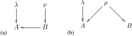
The image displays two separate directed acyclic graphs (DAGs), labeled (a) and (b), presented side-by-side. These diagrams are typical of those used in fields like statistics, machine learning, causal inference, or probabilistic graphical models to represent dependencies or causal relationships between variables. The nodes are represented by Greek and Latin letters, and the directed edges (arrows) indicate the direction of influence or conditional dependence.
### Components/Axes
The image contains two distinct diagrams with no shared axes, as they are not charts. The components are nodes and directed edges.
**Diagram (a) - Left Side:**
* **Nodes:** Four nodes labeled with the symbols: `λ` (lambda), `ν` (nu), `A`, and `B`.
* **Directed Edges (Arrows):**
1. An arrow from `λ` pointing downward to `A`.
2. An arrow from `ν` pointing downward to `B`.
3. An arrow from `B` pointing leftward to `A`.
**Diagram (b) - Right Side:**
* **Nodes:** Four nodes labeled with the symbols: `λ` (lambda), `μ` (mu), `A`, and `B`.
* **Directed Edges (Arrows):**
1. An arrow from `λ` pointing downward to `A`.
2. An arrow from `μ` pointing diagonally down-left to `A`.
3. An arrow from `μ` pointing diagonally down-right to `B`.
### Detailed Analysis
The analysis focuses on the structural relationships depicted in each graph.
**Diagram (a) Structure:**
* **Component Isolation:** The graph can be seen as having two source nodes (`λ`, `ν`) and two target/intermediate nodes (`A`, `B`).
* **Flow/Relationships:**
* Node `A` has two direct parents: `λ` and `B`. This means `A` is directly influenced by or dependent on both `λ` and `B`.
* Node `B` has one direct parent: `ν`. It is directly influenced by `ν`.
* There is a direct path from `ν` to `B` to `A`, indicating an indirect influence of `ν` on `A` via `B`.
* There is no direct edge between `λ` and `ν`, suggesting they are modeled as independent exogenous variables in this structure.
**Diagram (b) Structure:**
* **Component Isolation:** The graph has two source nodes (`λ`, `μ`) and two leaf nodes (`A`, `B`).
* **Flow/Relationships:**
* Node `A` has two direct parents: `λ` and `μ`. It is directly influenced by both.
* Node `B` has one direct parent: `μ`. It is directly influenced only by `μ`.
* Nodes `A` and `B` share a common parent, `μ`. This creates a "fork" structure where `μ` is a common cause of both `A` and `B`.
* There is no direct edge between `A` and `B`. Any association between them would be mediated through their common parent `μ`.
### Key Observations
1. **Structural Difference:** The primary difference between the two models is the relationship between nodes `A` and `B`. In (a), `B` is a direct cause of `A`. In (b), `A` and `B` are not directly connected but share a common cause (`μ`).
2. **Node Roles:** The Greek letters (`λ`, `ν`, `μ`) consistently act as source or exogenous variables (no incoming arrows), while the Latin letters (`A`, `B`) act as endogenous variables (have incoming arrows).
3. **Visual Layout:** Both diagrams use a top-down hierarchical layout for the source nodes, with edges flowing downward. The edge from `B` to `A` in diagram (a) is a notable horizontal connection.
### Interpretation
These diagrams are abstract representations of dependency structures. Their meaning is context-dependent, but common interpretations include:
* **Causal Models:** The arrows represent direct causal effects.
* In **(a)**, `ν` causes `B`, which in turn causes `A`. `λ` is another independent cause of `A`. To estimate the total causal effect of `ν` on `A`, one must account for the path through `B`.
* In **(b)**, `μ` is a common cause of both `A` and `B`. This structure explains why `A` and `B` might be statistically associated (correlated) without one causing the other. The association is "confounded" by `μ`. The effect of `λ` on `A` is independent of `B`.
* **Probabilistic Graphical Models (e.g., Bayesian Networks):** The arrows encode conditional independence assumptions.
* In **(a)**, the joint probability distribution factors as: `P(λ, ν, A, B) = P(λ) * P(ν) * P(B|ν) * P(A|λ, B)`. This implies that `A` is conditionally independent of `ν` given `B`.
* In **(b)**, the joint probability distribution factors as: `P(λ, μ, A, B) = P(λ) * P(μ) * P(A|λ, μ) * P(B|μ)`. This implies that `A` and `B` are conditionally independent given `μ`.
**Conclusion:** The image presents two fundamental graphical structures used to reason about relationships between variables. Diagram (a) shows a chain or mediation structure (`ν -> B -> A`), while diagram (b) shows a common cause or confounding structure (`μ -> A` and `μ -> B`). The choice between these models would have significant implications for analysis, prediction, and intervention in a technical application.