\n
## Diagram: Phase Space Transformation
### Overview
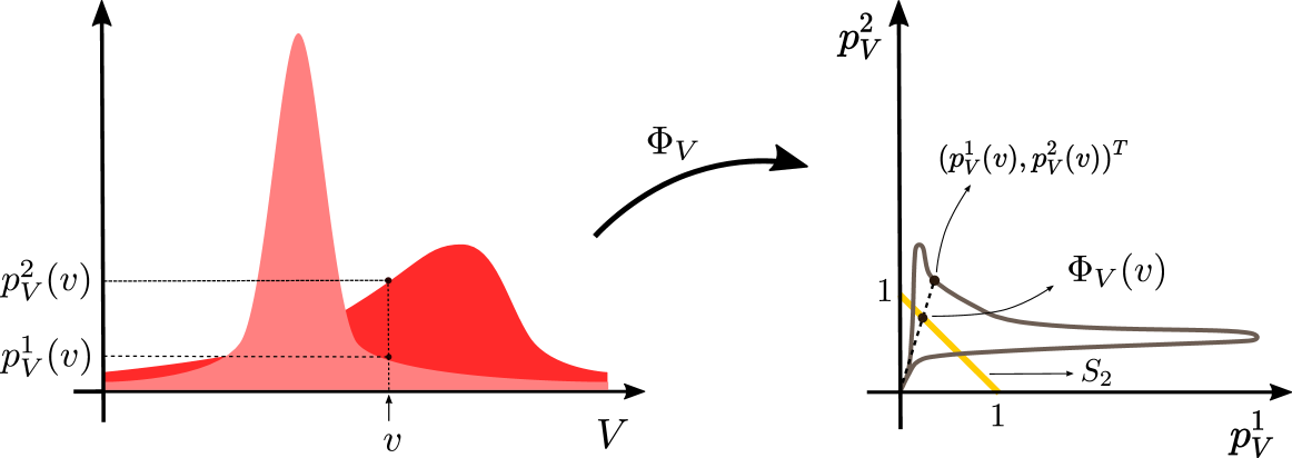
The image presents two diagrams illustrating a transformation, denoted as Φ<sub>V</sub>, within a phase space. The left diagram depicts a distribution of p<sub>V</sub><sup>2</sup>(v) and p<sub>V</sub><sup>1</sup>(v) as a function of velocity (v) and volume (V). The right diagram shows the transformation of this distribution in a space defined by p<sub>V</sub><sup>1</sup> and p<sub>V</sub><sup>2</sup>.
### Components/Axes
**Left Diagram:**
* **X-axis:** Labeled "V" (Volume).
* **Y-axis:** Labeled "p<sub>V</sub><sup>2</sup>(v)" (top) and "p<sub>V</sub><sup>1</sup>(v)" (bottom).
* **Vertical dashed line:** Marked with "v" (Velocity).
* **Shaded Area:** Represents a distribution, peaking around a specific velocity 'v'.
**Right Diagram:**
* **X-axis:** Labeled "p<sub>V</sub><sup>1</sup>". Scale ranges from approximately 0.5 to 1.5.
* **Y-axis:** Labeled "p<sub>V</sub><sup>2</sup>". Scale ranges from approximately 0.5 to 1.5.
* **Lines:** Several gray lines representing the transformation Φ<sub>V</sub>(v).
* **Yellow Line:** A single line representing the transformation Φ<sub>V</sub>(v) with a highlighted segment.
* **Black Line:** A line labeled "S<sub>2</sub>".
* **Text:** "(p<sub>V</sub><sup>1</sup>(v), p<sub>V</sub><sup>2</sup>(v))<sup>T</sup>" positioned near the top of the diagram.
* **Arrow:** A curved arrow labeled "Φ<sub>V</sub>" indicating the direction of the transformation.
### Detailed Analysis or Content Details
**Left Diagram:**
The distribution p<sub>V</sub><sup>1</sup>(v) and p<sub>V</sub><sup>2</sup>(v) is approximately symmetric around the velocity 'v'. The peak of the distribution is located at approximately V = 1 and p<sub>V</sub><sup>2</sup>(v) = 1.5, and p<sub>V</sub><sup>1</sup>(v) = 0.5. The distribution extends to lower values of p<sub>V</sub><sup>1</sup>(v) and higher values of p<sub>V</sub><sup>2</sup>(v).
**Right Diagram:**
The gray lines representing Φ<sub>V</sub>(v) appear to be curves that originate near (1,1) and bend upwards. The yellow line highlights a specific instance of the transformation. The highlighted segment starts at approximately (1, 1) and extends to approximately (1.2, 1.3). The line labeled S<sub>2</sub> is a vertical line at p<sub>V</sub><sup>1</sup> = 1. The text "(p<sub>V</sub><sup>1</sup>(v), p<sub>V</sub><sup>2</sup>(v))<sup>T</sup>" indicates a vector representation of the phase space coordinates.
### Key Observations
* The transformation Φ<sub>V</sub> maps points from the left diagram's distribution to curves in the right diagram's phase space.
* The highlighted segment of Φ<sub>V</sub>(v) suggests a specific trajectory or evolution of the system.
* The line S<sub>2</sub> might represent a constraint or boundary condition within the phase space.
* The distribution on the left is being mapped to a set of curves on the right.
### Interpretation
The diagrams illustrate a transformation of a probability distribution in phase space. The left diagram shows the initial distribution of momentum components (p<sub>V</sub><sup>1</sup> and p<sub>V</sub><sup>2</sup>) as a function of velocity and volume. The right diagram shows how this distribution is transformed by Φ<sub>V</sub>, mapping points in the original phase space to curves. This transformation could represent the evolution of a system over time, or a change in its state due to external forces. The line S<sub>2</sub> could represent a conserved quantity or a constraint on the system's motion. The vector notation "(p<sub>V</sub><sup>1</sup>(v), p<sub>V</sub><sup>2</sup>(v))<sup>T</sup>" suggests a mathematical formulation of the phase space coordinates. The diagrams are likely part of a theoretical framework describing the dynamics of a physical system, potentially in statistical mechanics or thermodynamics.