## Chart/Diagram Type: Probability Density Function Transformation
### Overview
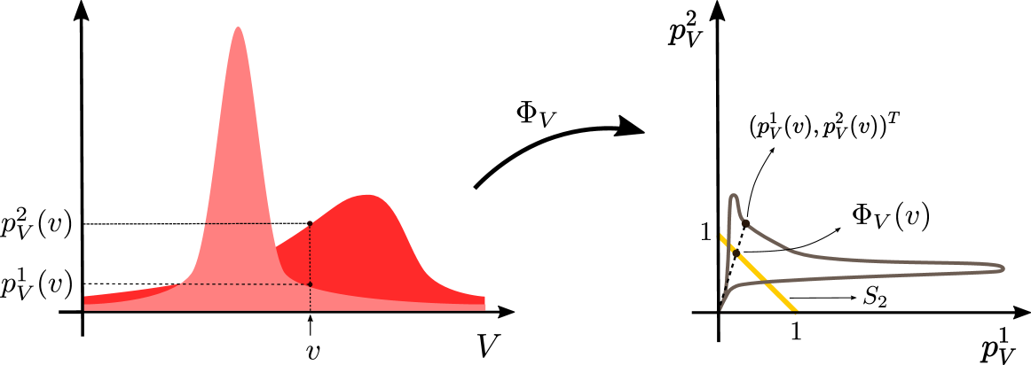
The image contains two graphical representations:
1. **Left Graph**: A probability density function (PDF) for a variable $ V $, showing two distinct peaks labeled $ p_1^V(v) $ and $ p_2^V(v) $.
2. **Right Graph**: A transformed distribution $ \Phi_V(v) $, derived from the original PDF via a function $ \Phi_V $, with a reference line $ S_2 $ and a coordinate system involving $ p_1^V $ and $ p_2^V $.
### Components/Axes
#### Left Graph
- **Vertical Axis**: Labeled $ p_2^V(v) $ and $ p_1^V(v) $, representing probability densities.
- **Horizontal Axis**: Labeled $ V $, representing the variable.
- **Key Elements**:
- Two red shaded peaks:
- $ p_1^V(v) $: Lower peak at a smaller $ V $ value.
- $ p_2^V(v) $: Higher peak at a larger $ V $ value.
- Dotted lines connecting peaks to their labels.
- Arrow labeled $ \Phi_V $ pointing to the right graph.
#### Right Graph
- **Vertical Axis**: Labeled $ p_2^V $, representing transformed probability densities.
- **Horizontal Axis**: Labeled $ p_1^V $, representing transformed probability densities.
- **Key Elements**:
- Curve labeled $ \Phi_V(v) $, starting at $ (1,1) $ and curving downward.
- Yellow line labeled $ S_2 $, starting at $ (1,1) $ and intersecting the $ \Phi_V(v) $ curve.
- Arrow labeled $ \Phi_V $ connecting the left and right graphs.
### Detailed Analysis
#### Left Graph
- The PDF for $ V $ has two distinct modes:
- $ p_1^V(v) $: Approximately 0.3 at $ V \approx 1.5 $.
- $ p_2^V(v) $: Approximately 0.7 at $ V \approx 3.0 $.
- The red shading indicates the probability density distribution.
#### Right Graph
- The transformation $ \Phi_V(v) $ maps the original distribution to a new space:
- At $ p_1^V = 1 $, $ p_2^V = 1 $, the curve starts.
- The curve $ \Phi_V(v) $ decreases non-linearly, suggesting a normalization or scaling operation.
- The line $ S_2 $ intersects $ \Phi_V(v) $ at $ p_1^V \approx 0.5 $, $ p_2^V \approx 0.8 $.
### Key Observations
1. **Bimodal Distribution**: The left graph shows two distinct peaks, indicating a bimodal distribution of $ V $.
2. **Transformation Behavior**: The right graph’s $ \Phi_V(v) $ curve suggests a non-linear transformation, possibly to reduce variance or align with a target distribution.
3. **Reference Line $ S_2 $**: The yellow line $ S_2 $ may represent a threshold or constraint in the transformed space.
### Interpretation
- The left graph demonstrates a bimodal distribution of $ V $, with $ p_2^V(v) $ being the dominant mode.
- The transformation $ \Phi_V $ maps this distribution into a new space where $ p_1^V $ and $ p_2^V $ are interdependent, as seen in the right graph.
- The line $ S_2 $ likely acts as a boundary or reference for the transformed probabilities, possibly indicating a condition for validity or optimization.
- The non-linear nature of $ \Phi_V(v) $ implies that the transformation is designed to handle the bimodality, potentially simplifying the distribution for further analysis.
### Notes on Uncertainty
- Exact numerical values for $ p_1^V(v) $ and $ p_2^V(v) $ are approximate, as the image lacks precise scale markers.
- The intersection point of $ S_2 $ and $ \Phi_V(v) $ is estimated based on visual alignment.