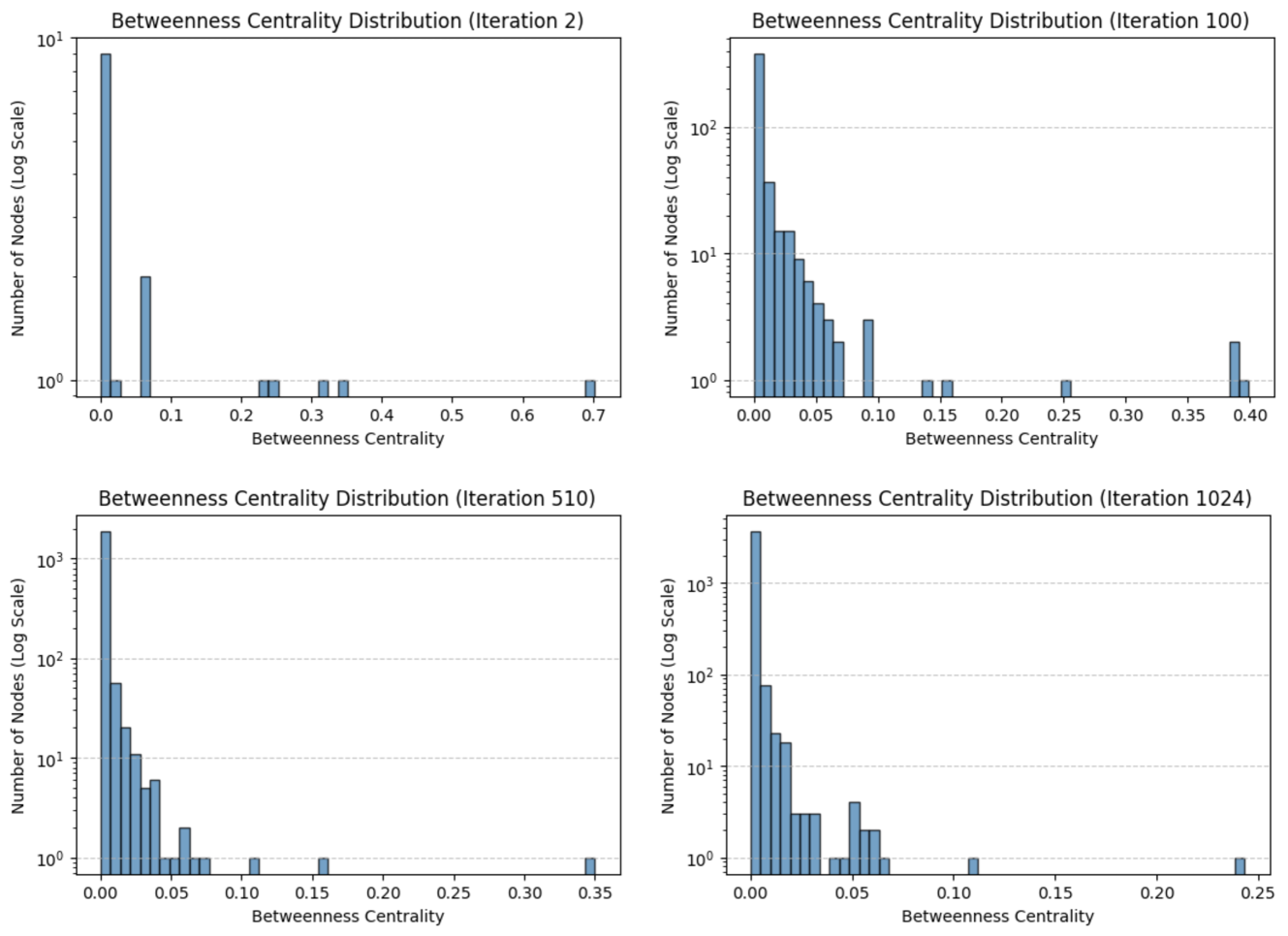
## Histogram Matrix: Betweenness Centrality Distribution over Iterations ### Overview This image presents a 2x2 grid of histograms illustrating the evolution of "Betweenness Centrality" across four distinct stages of a network simulation: Iteration 2, 100, 510, and 1024. Each plot displays the frequency distribution of nodes based on their betweenness centrality score. The Y-axis uses a logarithmic scale to accommodate the wide range of node counts, while the X-axis represents the centrality value. ### Components/Axes * **Common Y-Axis:** "Number of Nodes (Log Scale)". The scale varies per plot to accommodate the growth in the number of nodes. * **Common X-Axis:** "Betweenness Centrality". The range of values on this axis contracts as iterations increase. * **Layout:** * **Top-Left:** Iteration 2 * **Top-Right:** Iteration 100 * **Bottom-Left:** Iteration 510 * **Bottom-Right:** Iteration 1024 --- ### Detailed Analysis #### 1. Iteration 2 (Top-Left) * **Trend:** The distribution is sparse and fragmented. * **Data Points:** * The highest frequency is at the lowest centrality bin (near 0.0), with approximately 8-9 nodes. * A secondary cluster appears around 0.06 with approximately 3 nodes. * Isolated outliers exist at 0.23, 0.25, 0.32, 0.35, and a single node at 0.7. * **X-Axis Range:** 0.0 to 0.7. #### 2. Iteration 100 (Top-Right) * **Trend:** The distribution begins to resemble a power-law or heavy-tailed distribution. * **Data Points:** * A massive spike occurs at 0.0, with the count reaching approximately 400 nodes. * There is a rapid decay as centrality increases. * A small cluster of nodes is visible between 0.05 and 0.08. * Outliers are present at 0.14, 0.16, 0.25, 0.39, and 0.40. * **X-Axis Range:** 0.0 to 0.40. #### 3. Iteration 510 (Bottom-Left) * **Trend:** The power-law distribution becomes more pronounced and steeper. * **Data Points:** * The peak at 0.0 is significantly higher, reaching approximately 2,000 nodes. * The decay is very sharp. * Minor clusters appear between 0.03 and 0.06. * Isolated outliers are visible at 0.11, 0.16, and 0.35. * **X-Axis Range:** 0.0 to 0.35. #### 4. Iteration 1024 (Bottom-Right) * **Trend:** The distribution is highly concentrated at the lowest centrality values. * **Data Points:** * The peak at 0.0 is the highest of all plots, exceeding 3,000 nodes. * The distribution is extremely tight, with very few nodes having centrality above 0.05. * Small, sparse clusters appear between 0.04 and 0.06. * Isolated outliers are present at 0.11 and 0.24. * **X-Axis Range:** 0.0 to 0.25. --- ### Key Observations * **Node Growth:** The total number of nodes in the network increases dramatically as iterations progress, evidenced by the Y-axis scale shifting from 10^1 to 10^3. * **Centrality Contraction:** As the network grows, the maximum betweenness centrality value decreases (from 0.7 at Iteration 2 to 0.24 at Iteration 1024). * **Distribution Shape:** The data consistently follows a heavy-tailed distribution. The vast majority of nodes possess near-zero betweenness centrality, while a very small fraction of nodes act as high-centrality "hubs." ### Interpretation The data demonstrates the typical behavior of a growing network model (likely a preferential attachment model, such as Barabási-Albert). 1. **Network Expansion:** As the simulation progresses, the network adds more nodes. Because the Y-axis is logarithmic, the massive increase in the count of low-centrality nodes indicates that the network is expanding rapidly. 2. **Dilution of Centrality:** The contraction of the X-axis (the maximum centrality value dropping) suggests that as the network grows, the "betweenness" (the ability of a node to act as a bridge between others) is being distributed across a larger population. No single node maintains the high relative centrality seen in the early, smaller network. 3. **Structural Stability:** The consistency of the shape (the "L" shape of the histogram) suggests that the network maintains a stable topological structure (a scale-free network) even as it scales in size. The "rich-get-richer" phenomenon is present, but the relative influence of the "richest" nodes diminishes as the total node count increases.