TECHNICAL ASSET FINGERPRINT
613dca82f21b0dc3af8399ff
Click to view fullscreen
Press ESC or click to close
FOUND IN PAPERS
EXPERT: gemini-3.1-pro-preview VERSION 1
RUNTIME: gemini/gemini-3.1-pro-preview
INTEL_VERIFIED
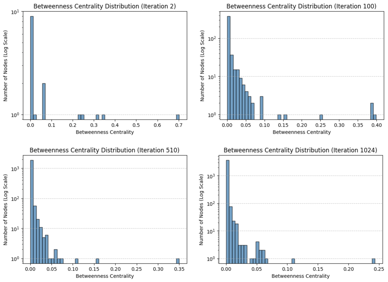
## Grid of Histograms: Evolution of Betweenness Centrality Distribution
### Overview
The image displays a 2x2 grid of histograms illustrating the "Betweenness Centrality Distribution" of a network across four distinct time steps or stages, labeled as "Iterations." The iterations shown are 2, 100, 510, and 1024. The charts demonstrate how the network's topology evolves, specifically showing a massive increase in the total number of nodes and a shift toward a highly skewed, power-law-like distribution where the vast majority of nodes have near-zero betweenness centrality. All text in the image is in English.
### Components/Axes
The image is divided into four quadrants (Top-Left, Top-Right, Bottom-Left, Bottom-Right). All four charts share the following structural components:
* **Chart Type:** Histogram (vertical bar charts).
* **Visual Style:** Light blue bars with dark borders. Horizontal dashed gridlines correspond to major Y-axis ticks.
* **X-axis Label:** "Betweenness Centrality" (Linear scale). Note: The maximum range of the X-axis changes across the iterations.
* **Y-axis Label:** "Number of Nodes (Log Scale)" (Logarithmic scale: $10^0$, $10^1$, $10^2$, $10^3$). Note: The maximum range of the Y-axis changes across the iterations as the network grows.
---
### Detailed Analysis
#### 1. Top-Left Chart: Iteration 2
* **Position:** Top-Left quadrant.
* **Title:** Betweenness Centrality Distribution (Iteration 2)
* **X-axis Range:** 0.0 to 0.7 (Markers at 0.0, 0.1, 0.2, 0.3, 0.4, 0.5, 0.6, 0.7).
* **Y-axis Range:** $10^0$ (1) to $10^1$ (10).
* **Visual Trend:** The distribution is sparse, indicating a very small network. There is a small cluster at 0.0, and a few individual nodes scattered across higher centrality values up to 0.7.
* **Data Points (Approximate):**
* ~0.00: ~9 nodes (just below the $10^1$ line)
* ~0.02: 1 node ($10^0$ line)
* ~0.06: ~2 nodes
* ~0.23: 1 node
* ~0.25: 1 node
* ~0.32: 1 node
* ~0.35: 1 node
* ~0.70: 1 node
#### 2. Top-Right Chart: Iteration 100
* **Position:** Top-Right quadrant.
* **Title:** Betweenness Centrality Distribution (Iteration 100)
* **X-axis Range:** 0.00 to 0.40 (Markers at 0.00, 0.05, 0.10, 0.15, 0.20, 0.25, 0.30, 0.35, 0.40). *Note the scale reduction from Iteration 2.*
* **Y-axis Range:** $10^0$ (1) to above $10^2$ (100).
* **Visual Trend:** A heavy right-skewed distribution emerges. A massive spike occurs at 0.00, trailing off rapidly. The network has grown significantly.
* **Data Points (Approximate):**
* ~0.00: ~350 nodes (bar extends well above $10^2$)
* ~0.01: ~40 nodes
* ~0.02: ~15 nodes
* ~0.03: ~15 nodes
* ~0.04: ~9 nodes
* ~0.05: ~6 nodes
* ~0.06: ~4 nodes
* ~0.07: ~2 nodes
* ~0.09: ~3 nodes
* ~0.14: 1 node
* ~0.16: 1 node
* ~0.25: 1 node
* ~0.39: ~2 nodes
* ~0.40: 1 node
#### 3. Bottom-Left Chart: Iteration 510
* **Position:** Bottom-Left quadrant.
* **Title:** Betweenness Centrality Distribution (Iteration 510)
* **X-axis Range:** 0.00 to 0.35 (Markers at 0.00, 0.05, 0.10, 0.15, 0.20, 0.25, 0.30, 0.35). *Scale reduction continues.*
* **Y-axis Range:** $10^0$ (1) to above $10^3$ (1000).
* **Visual Trend:** Extreme right skew. The peak at zero centrality has grown exponentially compared to Iteration 100.
* **Data Points (Approximate):**
* ~0.00: ~3000 nodes (bar extends significantly above $10^3$)
* ~0.01: ~60 nodes
* ~0.02: ~20 nodes
* ~0.03: ~10 nodes
* ~0.04: ~5 nodes
* ~0.05: ~6 nodes
* ~0.06: 1 node
* ~0.07: ~2 nodes
* ~0.08: 1 node
* ~0.11: 1 node
* ~0.16: 1 node
* ~0.35: 1 node
#### 4. Bottom-Right Chart: Iteration 1024
* **Position:** Bottom-Right quadrant.
* **Title:** Betweenness Centrality Distribution (Iteration 1024)
* **X-axis Range:** 0.00 to 0.25 (Markers at 0.00, 0.05, 0.10, 0.15, 0.20, 0.25). *Maximum centrality is now much lower.*
* **Y-axis Range:** $10^0$ (1) to above $10^3$ (1000).
* **Visual Trend:** The distribution solidifies its extreme right-skewed shape. The vast majority of the network's nodes have near-zero betweenness.
* **Data Points (Approximate):**
* ~0.00: ~4500 nodes (highest peak across all charts)
* ~0.01: ~80 nodes
* ~0.02: ~25 nodes
* ~0.03: ~18 nodes
* ~0.04: ~3 nodes
* ~0.05: ~3 nodes
* ~0.06: 1 node
* ~0.07: ~4 nodes
* ~0.08: ~2 nodes
* ~0.09: ~2 nodes
* ~0.10: 1 node
* ~0.13: 1 node
* ~0.24: 1 node
---
### Key Observations
1. **Explosive Node Growth:** The Y-axis maximum increases from $10^1$ (Iteration 2) to well over $10^3$ (Iteration 1024). The network is actively growing over time, adding thousands of nodes.
2. **Decreasing Maximum Centrality:** In Iteration 2, the highest betweenness centrality is ~0.7. By Iteration 1024, the highest value has shrunk to ~0.24. The X-axis scale compresses accordingly in each subsequent chart.
3. **Solidification of Skew:** The distribution shifts from a sparse, somewhat random scattering (Iteration 2) to a highly defined, long-tail distribution (Iterations 510 and 1024).
### Interpretation
Applying Peircean abductive reasoning to these visual trends reveals the underlying mechanics of the network being modeled:
* **Network Growth Model:** The data strongly suggests a generative network model (such as the Barabási–Albert model of preferential attachment). We are watching a network grow from a tiny seed (Iteration 2) into a massive complex system (Iteration 1024).
* **The Meaning of the Zero-Peak:** Betweenness centrality measures how often a node acts as a bridge along the shortest path between two other nodes. The massive, exponentially growing spike at 0.00 indicates that as the network grows, almost all *new* nodes are added to the periphery (leaf nodes). They do not act as bridges for any other nodes.
* **Dilution of Centrality:** The fact that the *maximum* betweenness centrality drops from 0.7 to 0.24 is highly significant. In a tiny network (Iteration 2), a single central node might be the *only* bridge between two halves of the network, giving it a very high relative centrality score (0.7). As the network grows to thousands of nodes (Iteration 1024), it becomes denser. More alternative paths are created. Even the most critical "hub" nodes now share the bridging load with other pathways, diluting their individual betweenness score relative to the whole network, capping out at ~0.24.
* **Conclusion:** The charts successfully visualize the emergence of a scale-free or complex network topology, characterized by a few highly connected hubs (the long tail on the right) and a massive majority of peripheral, low-influence nodes (the massive spike on the left).
DECODING INTELLIGENCE...