## Histograms: Betweenness Centrality Distribution
### Overview
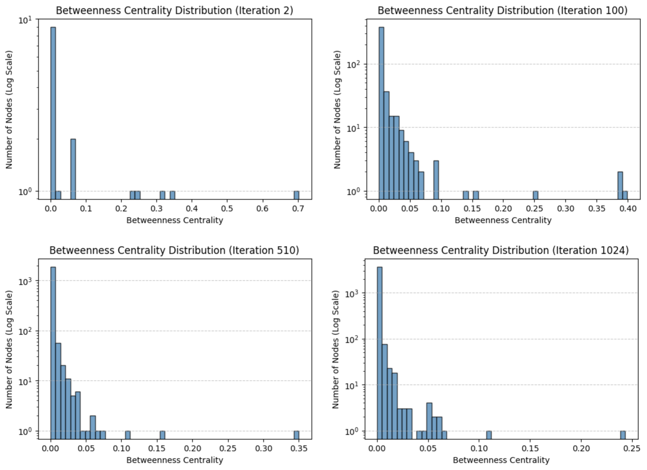
The image presents four histograms, each depicting the distribution of Betweenness Centrality values for a network at different iterations (2, 100, 510, and 1024). The y-axis of each histogram represents the "Number of Nodes" on a logarithmic scale, while the x-axis represents the "Betweenness Centrality" value. All histograms share the same axes scales.
### Components/Axes
* **Title:** "Betweenness Centrality Distribution (Iteration X)" where X is the iteration number (2, 100, 510, 1024). Positioned at the top-center of each individual histogram.
* **X-axis Label:** "Betweenness Centrality".
* **Y-axis Label:** "Number of Nodes (Log Scale)".
* **Scale (Y-axis):** Logarithmic, ranging from 10<sup>1</sup> to 10<sup>3</sup>.
* **Scale (X-axis):** Linear, ranging from 0.0 to approximately 0.7 (varies slightly between histograms).
* **Histograms:** Each histogram is composed of a series of blue bars representing the frequency of nodes within specific Betweenness Centrality ranges.
### Detailed Analysis or Content Details
**Histogram 1: Iteration 2**
* The histogram is heavily skewed to the left.
* The highest frequency of nodes occurs at very low Betweenness Centrality values (close to 0.0).
* There are a few nodes with Betweenness Centrality values up to approximately 0.7.
* Approximate counts (reading from the log scale):
* Betweenness Centrality 0.0 - 0.1: ~500 nodes
* Betweenness Centrality 0.1 - 0.2: ~100 nodes
* Betweenness Centrality 0.2 - 0.3: ~30 nodes
* Betweenness Centrality 0.3 - 0.4: ~10 nodes
* Betweenness Centrality 0.4 - 0.5: ~5 nodes
* Betweenness Centrality 0.5 - 0.6: ~2 nodes
* Betweenness Centrality 0.6 - 0.7: ~1 node
**Histogram 2: Iteration 100**
* The histogram shows a more pronounced distribution compared to Iteration 2.
* The peak frequency is still at low Betweenness Centrality values, but the distribution extends further to the right.
* Approximate counts:
* Betweenness Centrality 0.0 - 0.05: ~800 nodes
* Betweenness Centrality 0.05 - 0.1: ~400 nodes
* Betweenness Centrality 0.1 - 0.15: ~200 nodes
* Betweenness Centrality 0.15 - 0.2: ~100 nodes
* Betweenness Centrality 0.2 - 0.25: ~50 nodes
* Betweenness Centrality 0.25 - 0.3: ~20 nodes
* Betweenness Centrality 0.3 - 0.35: ~10 nodes
* Betweenness Centrality 0.35 - 0.4: ~5 nodes
**Histogram 3: Iteration 510**
* The distribution continues to shift towards higher Betweenness Centrality values.
* The peak is narrower and lower than in Iteration 100.
* Approximate counts:
* Betweenness Centrality 0.0 - 0.05: ~600 nodes
* Betweenness Centrality 0.05 - 0.1: ~300 nodes
* Betweenness Centrality 0.1 - 0.15: ~150 nodes
* Betweenness Centrality 0.15 - 0.2: ~75 nodes
* Betweenness Centrality 0.2 - 0.25: ~30 nodes
* Betweenness Centrality 0.25 - 0.3: ~15 nodes
* Betweenness Centrality 0.3 - 0.35: ~5 nodes
**Histogram 4: Iteration 1024**
* The distribution is further shifted to the right, with a more concentrated peak at lower values.
* The maximum Betweenness Centrality value observed is approximately 0.25.
* Approximate counts:
* Betweenness Centrality 0.0 - 0.05: ~700 nodes
* Betweenness Centrality 0.05 - 0.1: ~400 nodes
* Betweenness Centrality 0.1 - 0.15: ~200 nodes
* Betweenness Centrality 0.15 - 0.2: ~100 nodes
* Betweenness Centrality 0.2 - 0.25: ~50 nodes
### Key Observations
* The distribution of Betweenness Centrality values changes significantly over the iterations.
* Initially (Iteration 2), most nodes have very low Betweenness Centrality.
* As the iterations progress, the distribution shifts towards higher values, indicating that more nodes become central to the network's flow.
* The peak of the distribution consistently remains at low Betweenness Centrality, suggesting that a large proportion of nodes still have relatively low centrality even after many iterations.
* The range of Betweenness Centrality values decreases with increasing iterations, suggesting the network is converging.
### Interpretation
The data suggests that the network is evolving over the iterations, with nodes gradually becoming more central. The shift in the distribution of Betweenness Centrality indicates that the network's structure is changing, potentially leading to the formation of more critical pathways and influential nodes. The convergence of the distribution (decreasing range of values) suggests that the network is stabilizing, and the centrality of nodes is becoming more defined. The logarithmic scale on the y-axis emphasizes the large number of nodes with low Betweenness Centrality, highlighting the hierarchical nature of the network. The decreasing number of nodes with high Betweenness Centrality as iterations increase suggests that the network is becoming more efficient, with fewer nodes controlling the flow of information or resources. This could be due to a process of network optimization or the emergence of a dominant core.