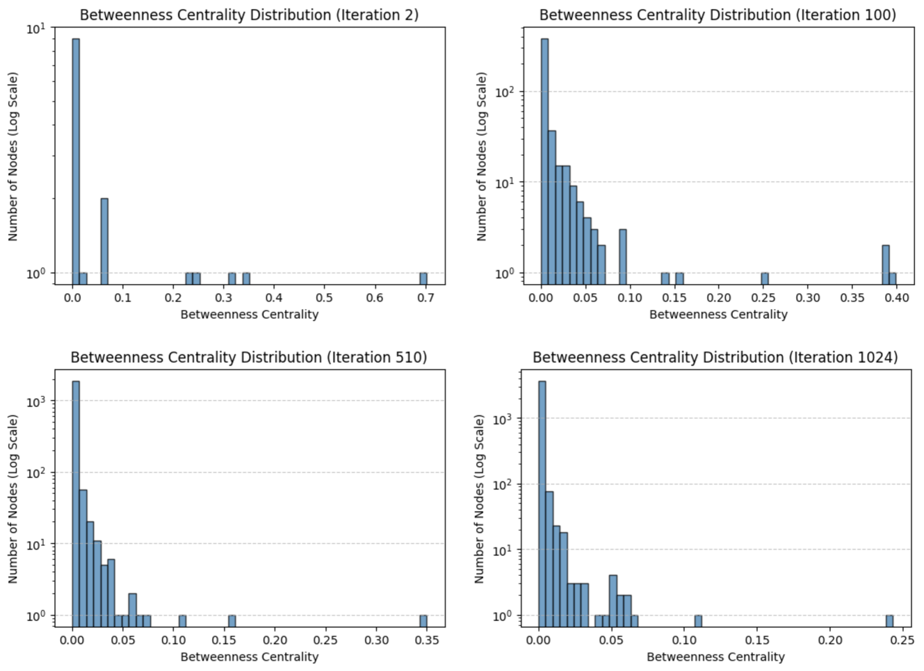
## Histograms: Betweenness Centrality Distribution Across Iterations ### Overview The image displays a 2x2 grid of four histograms, each titled "Betweenness Centrality Distribution" followed by an iteration number in parentheses. The charts visualize how the distribution of betweenness centrality values for nodes in a network evolves over time (iterations). All charts use a logarithmic scale for the vertical axis (Number of Nodes) and a linear scale for the horizontal axis (Betweenness Centrality). ### Components/Axes * **Chart Type:** Four separate histograms (bar charts). * **Titles:** * Top-Left: "Betweenness Centrality Distribution (Iteration 2)" * Top-Right: "Betweenness Centrality Distribution (Iteration 100)" * Bottom-Left: "Betweenness Centrality Distribution (Iteration 510)" * Bottom-Right: "Betweenness Centrality Distribution (Iteration 1024)" * **X-Axis (All Charts):** Label: "Betweenness Centrality". The scale range varies per chart. * **Y-Axis (All Charts):** Label: "Number of Nodes (Log Scale)". The scale is logarithmic (base 10), with major grid lines at powers of 10 (10⁰, 10¹, 10², 10³). * **Visual Elements:** Blue bars with black outlines represent the frequency (node count) for bins of betweenness centrality values. Dashed horizontal grid lines correspond to the logarithmic y-axis ticks. ### Detailed Analysis **1. Iteration 2 (Top-Left)** * **X-Axis Range:** 0.0 to 0.7. * **Distribution:** Extremely sparse. The vast majority of nodes have a betweenness centrality near 0.0. * **Key Data Points (Approximate):** * A dominant bar at ~0.0 centrality reaches just below 10¹ (≈8-9 nodes). * A smaller bar at ~0.06 centrality has a height of ~2-3 nodes. * Isolated, single-node bars (height = 10⁰) appear at approximately 0.23, 0.31, 0.34, and 0.69. * **Trend:** The distribution is highly skewed with a few outlier nodes possessing very high centrality. **2. Iteration 100 (Top-Right)** * **X-Axis Range:** 0.00 to 0.40. * **Distribution:** More nodes are present, forming a clearer, right-skewed distribution. The maximum centrality value has decreased. * **Key Data Points (Approximate):** * The tallest bar at ~0.00 centrality is between 10² and 10³ (≈300-400 nodes). * A rapid decay follows: bars at ~0.01 (≈40 nodes), ~0.02 (≈15 nodes), ~0.03 (≈10 nodes), ~0.04 (≈5 nodes), ~0.05 (≈3 nodes). * A small cluster appears around 0.09 (≈3 nodes). * Isolated single-node bars are at ~0.14, ~0.15, ~0.25, and ~0.39. * **Trend:** The network has grown, and centrality is more distributed, though still heavily concentrated near zero. **3. Iteration 510 (Bottom-Left)** * **X-Axis Range:** 0.00 to 0.35. * **Distribution:** The number of nodes has increased by an order of magnitude. The distribution is smoother but still strongly right-skewed. * **Key Data Points (Approximate):** * The peak at ~0.00 centrality is now above 10³ (≈1500-2000 nodes). * The decay is more gradual: bars at ~0.01 (≈60 nodes), ~0.02 (≈20 nodes), ~0.03 (≈10 nodes), ~0.04 (≈5 nodes), ~0.05 (≈2 nodes). * A small bump appears at ~0.06 (≈2 nodes). * Isolated single-node bars are at ~0.11, ~0.16, and ~0.35. * **Trend:** Continued network growth. The "tail" of the distribution (nodes with moderate centrality) is becoming more populated. **4. Iteration 1024 (Bottom-Right)** * **X-Axis Range:** 0.00 to 0.25. * **Distribution:** Similar in shape to Iteration 510, but the maximum centrality value has further decreased. The total node count appears similar or slightly higher. * **Key Data Points (Approximate):** * The peak at ~0.00 centrality is again above 10³ (≈2000-3000 nodes). * The decay pattern is consistent: bars at ~0.01 (≈80 nodes), ~0.02 (≈25 nodes), ~0.03 (≈15 nodes), ~0.04 (≈3 nodes), ~0.05 (≈4 nodes), ~0.06 (≈2 nodes). * Isolated single-node bars are at ~0.11 and ~0.24. * **Trend:** The distribution appears to be stabilizing. The network is large, and high betweenness centrality (above 0.1) is becoming increasingly rare for individual nodes. ### Key Observations 1. **Network Growth:** The total number of nodes (inferred from the area under the histogram and the y-axis peak) increases dramatically from Iteration 2 to Iteration 1024. 2. **Concentration at Zero:** In all iterations, the mode of the distribution is at or very near a betweenness centrality of 0.0, indicating most nodes lie on very few or no shortest paths between other nodes. 3. **Decreasing Maximum Centrality:** The highest observed betweenness centrality value decreases steadily across iterations: ~0.69 (It. 2) → ~0.39 (It. 100) → ~0.35 (It. 510) → ~0.24 (It. 1024). 4. **Distribution Shape Evolution:** The distribution evolves from a few extreme outliers (It. 2) to a smooth, rapidly decaying right-skewed distribution (It. 100 onwards), characteristic of many real-world networks. 5. **Sparse Tail:** Even in later iterations, the "tail" of the distribution (centrality > 0.1) is populated by only a handful of nodes, often just one. ### Interpretation This sequence of histograms likely depicts the evolution of a growing network model (e.g., a preferential attachment or spatial network model) where betweenness centrality is being recalculated at each major iteration. * **What the data suggests:** The data demonstrates a fundamental property of many evolving networks: as the network grows, the *relative* importance of any single node as a bridge (measured by betweenness centrality) tends to diminish for the vast majority of nodes. While new nodes are added, the "load" of being on shortest paths becomes more distributed. The decreasing maximum centrality suggests the network is becoming less reliant on a few critical "hub" nodes for global connectivity, potentially indicating increased robustness. * **How elements relate:** The four charts are snapshots in time. The shift in x-axis range and y-axis magnitude directly visualizes the network's growth and the changing statistical properties of its node centrality. The consistent log-scale y-axis allows for comparison of distribution shape across orders of magnitude in node count. * **Notable anomalies/trends:** The most striking trend is the compression of the centrality range. The outlier node with centrality ~0.69 in Iteration 2 is a significant anomaly compared to later stages. Its disappearance suggests a major structural change in the network between Iteration 2 and 100, where the initial "bottleneck" structure was broken or diluted by subsequent growth. The stabilization between Iterations 510 and 1024 suggests the network may be approaching a steady-state statistical distribution for betweenness centrality.