## Histograms: Betweenness Centrality Distribution Across Iterations
### Overview
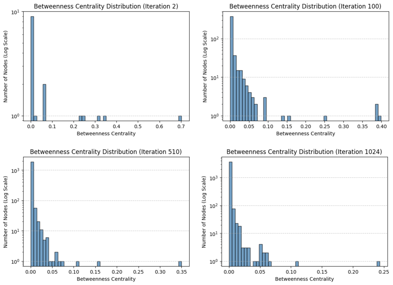
The image contains four histograms comparing the distribution of betweenness centrality values across network nodes at different computational iterations (Iteration 2, 100, 510, and 1024). All histograms use a logarithmic scale for the y-axis (Number of Nodes) and a linear scale for the x-axis (Betweenness Centrality). The data shows how node centrality distributions evolve as the algorithm progresses through iterations.
### Components/Axes
- **X-axis**: Betweenness Centrality (ranges from 0.0 to 0.7 in all charts)
- **Y-axis**: Number of Nodes (log scale: 10⁰ to 10³)
- **Legend**: Not explicitly present, but colors are consistent across charts (blue bars)
- **Titles**: Each subplot is labeled with "Betweenness Centrality Distribution (Iteration X)" where X = 2, 100, 510, 1024
### Detailed Analysis
#### Iteration 2
- **Peaks**:
- 0.0: ~10 nodes
- 0.05: ~5 nodes
- **Trend**: Sharp drop after 0.05, with minimal values beyond 0.1
- **Spread**: Concentrated near 0.0
#### Iteration 100
- **Peaks**:
- 0.0: ~100 nodes
- 0.05: ~50 nodes
- 0.1: ~10 nodes
- **Trend**: Broader distribution than Iteration 2, with secondary peaks at 0.05 and 0.1
- **Spread**: Extends to 0.15
#### Iteration 510
- **Peaks**:
- 0.0: ~1,000 nodes
- 0.05: ~100 nodes
- 0.1: ~50 nodes
- **Trend**: Further concentration near 0.0, with smaller peaks at 0.05 and 0.1
- **Spread**: Extends to 0.15
#### Iteration 1024
- **Peaks**:
- 0.0: ~1,000 nodes
- 0.05: ~100 nodes
- 0.075: ~50 nodes
- 0.1: ~25 nodes
- **Trend**: Highest concentration at 0.0, with gradual decay toward 0.1
- **Spread**: Extends to 0.25
### Key Observations
1. **Logarithmic Scale Impact**: The y-axis scaling emphasizes differences in node counts across orders of magnitude.
2. **Iteration Progression**:
- Early iterations (2, 100) show broader distributions.
- Later iterations (510, 1024) exhibit sharper concentration near 0.0.
3. **Centrality Decay**: Nodes with higher betweenness centrality (>0.1) consistently represent smaller fractions of the network across all iterations.
4. **Stability**: The highest peak (0.0) remains dominant across all iterations, suggesting a core of highly central nodes persists.
### Interpretation
The data demonstrates that as the algorithm iterates, the network's betweenness centrality distribution becomes increasingly polarized:
- **Early iterations** (2, 100) suggest a more heterogeneous network with multiple moderately central nodes.
- **Later iterations** (510, 1024) indicate convergence toward a network structure dominated by a small group of highly central nodes (near 0.0), with rapid decay in centrality values for most nodes.
This pattern aligns with expectations for betweenness centrality in dynamic networks, where repeated computations may stabilize around a core-periphery structure. The logarithmic y-axis is critical for visualizing the exponential decay in node counts at higher centrality values, which would be less apparent on a linear scale.