## Line Chart: Probability Distribution P(q) at T = 0.31, Instance 2
### Overview
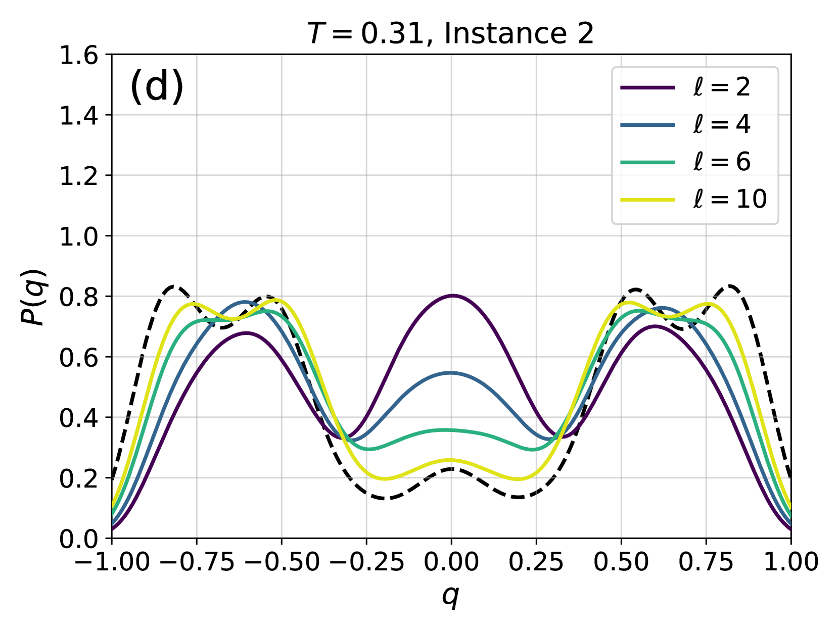
The chart displays the probability distribution \( P(q) \) as a function of \( q \) for four distinct values of \( \ell \) (2, 4, 6, 10) at a fixed temperature \( T = 0.31 \). A dashed black reference line is included for comparison. The y-axis (\( P(q) \)) ranges from 0 to 1.6, while the x-axis (\( q \)) spans from -1.00 to 1.00.
### Components/Axes
- **X-axis (q)**: Labeled with values from -1.00 to 1.00 in increments of 0.25.
- **Y-axis (P(q))**: Labeled with values from 0.0 to 1.6 in increments of 0.2.
- **Legend**: Located in the top-right corner, associating colors with \( \ell \) values:
- Purple: \( \ell = 2 \)
- Blue: \( \ell = 4 \)
- Teal: \( \ell = 6 \)
- Yellow: \( \ell = 10 \)
- **Title**: "T = 0.31, Instance 2" at the top of the chart.
### Detailed Analysis
1. **Dashed Black Line (Reference)**:
- Peaks at \( q \approx -0.5 \) and \( q \approx 0.5 \), with \( P(q) \approx 1.2 \).
- Symmetric about \( q = 0 \), forming a bimodal distribution.
2. **Solid Lines (by \( \ell \))**:
- **Purple (\( \ell = 2 \))**:
- Peaks at \( q \approx -0.5 \) and \( q \approx 0.5 \), with \( P(q) \approx 0.8 \).
- Slightly broader than the dashed line.
- **Blue (\( \ell = 4 \))**:
- Peaks at \( q \approx -0.5 \) and \( q \approx 0.5 \), with \( P(q) \approx 0.7 \).
- Broader than \( \ell = 2 \), with reduced amplitude.
- **Teal (\( \ell = 6 \))**:
- Peaks at \( q \approx -0.5 \) and \( q \approx 0.5 \), with \( P(q) \approx 0.5 \).
- Further reduced amplitude and broader spread.
- **Yellow (\( \ell = 10 \))**:
- Peaks at \( q \approx -0.5 \) and \( q \approx 0.5 \), with \( P(q) \approx 0.4 \).
- Flattest distribution, minimal amplitude.
### Key Observations
- All lines exhibit bimodal symmetry around \( q = 0 \), mirroring the dashed reference line.
- As \( \ell \) increases, the peaks of \( P(q) \) decrease in height and broaden, indicating reduced probability concentration at \( q = \pm 0.5 \).
- The dashed line (\( \ell \to \infty \)?) serves as an upper bound for \( P(q) \).
### Interpretation
The chart suggests that \( \ell \) inversely correlates with the sharpness of the \( P(q) \) distribution. Higher \( \ell \) values flatten the distribution, implying a transition from localized to delocalized behavior in the system. The temperature \( T = 0.31 \) and "Instance 2" label hint at a controlled experimental or simulated scenario, possibly studying phase transitions or critical phenomena where \( \ell \) modulates system dynamics. The dashed line may represent an idealized or theoretical limit (e.g., infinite \( \ell \)), against which finite-\( \ell \) results are compared.