## Diagram: Mathematical Transformation Flowchart
### Overview
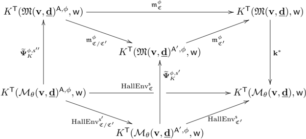
The image depicts a complex mathematical flowchart illustrating transformations between operators and functions. It involves multiple instances of the operator $ K^T$ applied to modified versions of $\mathcal{M}(v, d)$ and $\mathcal{M}_\theta(v, d)$, with parameters $\phi, w, \epsilon, \epsilon'$, and mappings denoted by arrows labeled with terms like $m_\phi$, $\text{HallEnv}$, and $\Psi_K$.
### Components/Axes
- **Key Labels**:
- $K^T(\mathcal{M}(v, d)^{A,\phi}, w)$: Top-left node, representing a transformed version of $\mathcal{M}(v, d)$ with parameters $A, \phi, w$.
- $K^T(\mathcal{M}(v, d), w)$: Top-right node, a simpler transformation of $\mathcal{M}(v, d)$.
- $K^T(\mathcal{M}_\theta(v, d)^{A,\phi}, w)$: Bottom-left node, similar to the top-left but with $\mathcal{M}_\theta$.
- $K^T(\mathcal{M}_\theta(v, d), w)$: Bottom-right node, a simpler transformation of $\mathcal{M}_\theta$.
- **Arrows and Mappings**:
- Horizontal arrows labeled $m_\phi$, $m_{\phi/\epsilon'}$, and $\text{HallEnv}_\phi$ connect nodes, suggesting parameter adjustments or environmental mappings.
- Vertical arrows labeled $\Psi_K$ and $k^*$ indicate projections or evaluations.
- **Notable Symbols**:
- $\Psi_K$: Appears on vertical arrows, likely a projection operator.
- $k^*$: Denotes a specific kernel or function.
### Detailed Analysis
- **Top-Left to Top-Right**:
$K^T(\mathcal{M}(v, d)^{A,\phi}, w) \xrightarrow{m_\phi} K^T(\mathcal{M}(v, d), w)$: A transformation where $\mathcal{M}(v, d)$ is adjusted by $A, \phi$, then simplified.
- **Top-Right to Bottom-Right**:
$K^T(\mathcal{M}(v, d), w) \xrightarrow{k^*} K^T(\mathcal{M}_\theta(v, d), w)$: A mapping involving $k^*$, possibly a kernel substitution.
- **Bottom-Left to Bottom-Right**:
$K^T(\mathcal{M}_\theta(v, d)^{A,\phi}, w) \xrightarrow{\text{HallEnv}_{\epsilon/\epsilon'}} K^T(\mathcal{M}_\theta(v, d), w)$: Adjustments via $\text{HallEnv}$, likely contextual or environmental factors.
- **Vertical Arrows**:
- $\Psi_K$: Connects top-left and bottom-left nodes, suggesting a shared projection.
- $k^*$: Links top-right and bottom-right nodes, indicating a consistent kernel.
### Key Observations
- The diagram emphasizes **parameterized transformations** of $\mathcal{M}(v, d)$ and $\mathcal{M}_\theta(v, d)$, with $\phi, w, \epsilon, \epsilon'$ as critical variables.
- $\text{HallEnv}$ and $m_\phi$ suggest **contextual or environmental adjustments** to the transformations.
- $\Psi_K$ and $k^*$ act as **bridging operators**, linking different stages of the flow.
### Interpretation
This flowchart likely models a **multi-stage mathematical process** where:
1. **Initial transformations** ($K^T$) are applied to $\mathcal{M}(v, d)$ and $\mathcal{M}_\theta(v, d)$ with parameters $A, \phi, w$.
2. **Adjustments** ($m_\phi, \text{HallEnv}$) refine these transformations based on contextual factors ($\epsilon, \epsilon'$).
3. **Projections** ($\Psi_K$) and **kernels** ($k^*$) unify or evaluate the results across different stages.
The diagram may represent a **machine learning or signal processing framework**, where $\mathcal{M}$ and $\mathcal{M}_\theta$ are models, $\phi$ and $w$ are hyperparameters, and $\text{HallEnv}$ accounts for environmental noise or constraints. The use of $k^*$ suggests a **standardized kernel** for consistency in later stages.
No numerical data or trends are present; the focus is on symbolic relationships and structural dependencies.