## Network Diagrams (12 Node-Link Graphs)
### Overview
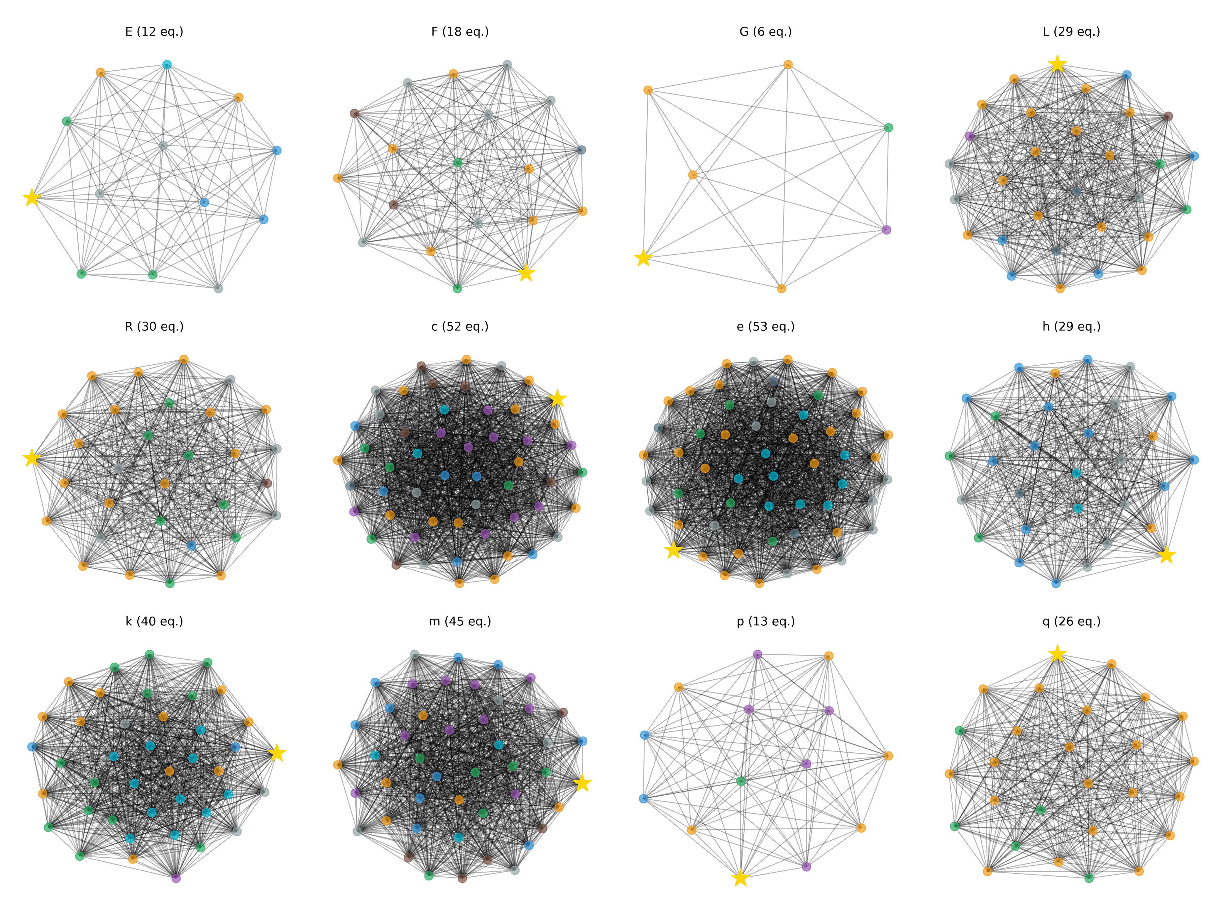
The image displays a 3×4 grid of **node-link network diagrams**, each labeled with a letter and a number in parentheses (e.g., *“E (12 eq.)”*). Each diagram visualizes connections (edges) between colored nodes (yellow star, green, blue, orange, purple, gray), with the number of *“eq.”* (likely “elements” or “nodes”) indicated in the label.
### Components/Axes
- **Labels**: Each graph has a title above it (e.g., *“E (12 eq.)”*), specifying a letter and the number of *“eq.”* (nodes/elements).
- Top row: *E (12 eq.)*, *F (18 eq.)*, *G (6 eq.)*, *L (29 eq.)*
- Middle row: *R (30 eq.)*, *c (52 eq.)*, *e (53 eq.)*, *h (29 eq.)*
- Bottom row: *k (40 eq.)*, *m (45 eq.)*, *p (13 eq.)*, *q (26 eq.)*
- **Nodes**: Colored circles (yellow star, green, blue, orange, purple, gray) representing entities (e.g., nodes in a network).
- **Edges**: Black lines connecting nodes, indicating relationships (e.g., interactions, connections).
- **Spatial Layout**: 3 rows (top, middle, bottom) and 4 columns (left to right), with each graph in a distinct cell.
### Detailed Analysis
#### Top Row (Left to Right):
- **E (12 eq.)**: ~12 nodes (yellow star, green, blue, orange, gray). Edges are moderately dense, connecting most nodes.
- **F (18 eq.)**: ~18 nodes (additional colors: purple, brown). Edges are denser than *E*, with more connections.
- **G (6 eq.)**: ~6 nodes (yellow star, green, orange, purple). Edges are sparse, with few connections.
- **L (29 eq.)**: ~29 nodes (dense, many colors). Edges are very dense, forming a complex network.
#### Middle Row (Left to Right):
- **R (30 eq.)**: ~30 nodes (dense, yellow star). Edges are highly dense, with many connections.
- **c (52 eq.)**: ~52 nodes (extremely dense, many colors). Edges are nearly a solid mass, indicating high connectivity.
- **e (53 eq.)**: ~53 nodes (most dense, yellow star). Edges are extremely dense, with minimal visible gaps.
- **h (29 eq.)**: ~29 nodes (dense, yellow star). Edges are dense, similar to *L* but with a different node distribution.
#### Bottom Row (Left to Right):
- **k (40 eq.)**: ~40 nodes (dense, yellow star). Edges are dense, with a mix of node colors.
- **m (45 eq.)**: ~45 nodes (dense, yellow star). Edges are dense, with a complex node arrangement.
- **p (13 eq.)**: ~13 nodes (sparser, yellow star). Edges are less dense than *k/m*, with fewer connections.
- **q (26 eq.)**: ~26 nodes (dense, yellow star). Edges are dense, with a balanced node distribution.
### Key Observations
- **Density Trend**: As the number of *“eq.”* increases (e.g., *G (6)* → *e (53)*), edge density (connectivity) increases, showing more complex networks.
- **Node Colors**: The yellow star is a consistent prominent node (likely a central/key node) in all graphs. Other colors (green, blue, orange, purple, gray) represent different node types.
- **Sparse vs. Dense**: Graphs with fewer *“eq.”* (*G (6)*, *p (13)*) have sparser edges, while those with more (*c (52)*, *e (53)*) are extremely dense.
### Interpretation
These diagrams likely represent **network structures** (e.g., social networks, biological pathways, or system interactions) where nodes are entities and edges are relationships. The *“eq.”* count suggests the number of nodes/elements, with higher counts indicating more complex systems. The yellow star may denote a critical node (e.g., a hub or central component). The increasing density with more nodes implies that larger networks have more interconnected elements, reflecting real-world systems where more components lead to more interactions. Sparse graphs (*G*, *p*) might represent simpler systems or subsets of larger networks.
(Note: No numerical data tables or explicit text blocks are present; the analysis focuses on network structure, node/edge relationships, and trends in connectivity.)