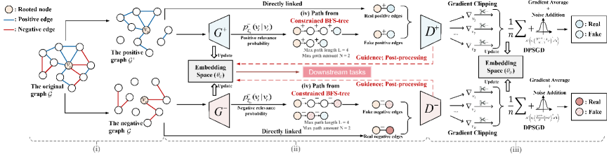
# Technical Document Extraction: Graph Neural Network Architecture Diagram
This document provides a detailed technical extraction of the provided image, which illustrates a Generative Adversarial Network (GAN) framework for graph embedding, specifically handling positive and negative edges with Differential Privacy (DPSGD).
## 1. Legend and Symbol Definitions
Located at the top-left of the image:
* **Tan circle with center dot**: Rooted node ($v_r$)
* **Blue line**: Positive edge
* **Red line**: Negative edge
Located at the far right (Discriminator outputs):
* **Solid Blue circle**: Real positive edge
* **Patterned Blue circle**: Fake positive edge
* **Solid Red circle**: Real negative edge
* **Patterned Red circle**: Fake negative edge
---
## 2. Component Segmentation and Flow
The diagram is divided into three primary horizontal stages, labeled at the bottom as (i), (ii), and (iii).
### Stage (i): Graph Decomposition
* **Input**: "The original graph $\mathcal{G}$" containing a central rooted node $v_r$ connected by both blue (positive) and red (negative) edges.
* **Process**: The original graph is split into two distinct subgraphs:
1. **The positive graph $\mathcal{G}^+$**: Contains only nodes and blue edges.
2. **The negative graph $\mathcal{G}^-$**: Contains only nodes and red edges.
### Stage (ii): Generative Process and Path Sampling
This stage describes the dual generator architecture ($G^+$ and $G^-$).
* **Embedding Space ($\theta_G$)**: A central block that provides parameters to and receives updates from the generators.
* **Positive Path Generation ($G^+$)**:
* **Input**: Data from the positive graph $\mathcal{G}^+$.
* **Function**: Calculates $P_{T_{v_r}}^+(v_i | v_r)$ (Positive relevance probability).
* **Output (iv)**: "Path from Constrained BFS-tree".
* Constraints: Max path length $L=4$, Max path amount $N=2$.
* Visual: Shows a sequence of nodes starting from a rooted node.
* **Result**: Produces "Fake positive edges" (represented by two light blue circles connected by a dashed line).
* **Direct Link**: "Real positive edges" are pulled directly from the positive graph $\mathcal{G}^+$ for comparison.
* **Negative Path Generation ($G^-$)**:
* **Input**: Data from the negative graph $\mathcal{G}^-$.
* **Function**: Calculates $P_{T_{v_r}}^-(v_i | v_r)$ (Negative relevance probability).
* **Output (iv)**: "Path from Constrained BFS-tree".
* Constraints: Max path length $L=4$, Max path amount $N=2$.
* **Result**: Produces "Fake negative edges" (represented by two light red circles connected by a dashed line).
* **Direct Link**: "Real negative edges" are pulled directly from the negative graph $\mathcal{G}^-$ for comparison.
* **Central Output**: A red arrow points from the Embedding Space to a box labeled **"Downstream tasks"**.
### Stage (iii): Discriminator and Differentially Private Training
This stage describes the evaluation and optimization process using Differentially Private Stochastic Gradient Descent (DPSGD).
* **Discriminators ($D^+$ and $D^-$)**:
* $D^+$ receives both Real and Fake positive edges.
* $D^-$ receives both Real and Fake negative edges.
* **Optimization Flow**:
1. **Gradient Calculation**: Gradients ($\nabla_{v_1}, \nabla_{v_2}, \dots, \nabla_{v_n}$) are computed.
2. **Gradient Clipping**: Represented by a scissor icon on the gradient arrows.
3. **DPSGD Process**:
* Formula: $\frac{1}{n} \sum + \text{Noise Addition}$
* The noise addition is visualized as a Gaussian distribution curve.
* Formula snippet: $\mathcal{N}(0, (\frac{2\sigma C}{n})^2 I)$
4. **Embedding Space ($\theta_D$)**: The processed gradients update a separate discriminator embedding space.
5. **Feedback Loop**: Red dashed arrows labeled **"Guidance: Post-processing"** flow from the Discriminators back to the Generators' Embedding Space ($\theta_G$).
---
## 3. Mathematical Notations and Labels
* **Root Node**: $v_r$
* **Probability Functions**: $P_{T_{v_r}}^+(v_i | v_r)$ and $P_{T_{v_r}}^-(v_i | v_r)$
* **Embedding Parameters**: $\theta_G$ (Generator) and $\theta_D$ (Discriminator)
* **Training Mechanism**: DPSGD (Differential Private Stochastic Gradient Descent)
* **BFS Constraints**: $L=4$ (Length), $N=2$ (Amount)
## 4. Summary of Logic and Trends
The system employs a **Symmetric Dual-GAN architecture**. The "Positive" and "Negative" branches mirror each other exactly in structure but process different edge types. The trend of the data flow is from left to right (Decomposition $\rightarrow$ Generation $\rightarrow$ Discrimination), with a critical feedback loop (Guidance) returning to the center to refine the embeddings. The inclusion of Gradient Clipping and Noise Addition indicates a focus on privacy-preserving graph representation learning.