## Diagram: Star Polygon and 3D Representation ### Overview The image presents two visualizations of a geometric structure. On the left, a 2D representation of a star polygon is shown. On the right, a 3D representation of a similar structure is displayed within a gridded coordinate system. Both visualizations use blue lines to connect adjacent vertices and red lines to connect non-adjacent vertices. Black dots mark the vertices of the structure. ### Components/Axes * **Left (2D Representation):** * Vertices: Represented by black dots. * Edges: Represented by blue lines connecting adjacent vertices. * Diagonals: Represented by red lines connecting non-adjacent vertices. * **Right (3D Representation):** * Vertices: Represented by black dots. * Edges: Represented by blue lines connecting adjacent vertices. * Diagonals: Represented by red lines connecting non-adjacent vertices. * Coordinate System: A 3D grid provides spatial context. The grid lines are light gray. ### Detailed Analysis * **Left (2D Representation):** * The polygon has 12 vertices. * The blue lines form the perimeter of the polygon. * The red lines connect each vertex to several non-adjacent vertices, creating a star-like pattern within the polygon. * **Right (3D Representation):** * The structure appears to be a polyhedron with 10 vertices. * The blue lines form the edges of the polyhedron. * The red lines connect vertices within the polyhedron, creating a complex network of diagonals. * The 3D grid provides a sense of depth and spatial orientation. ### Key Observations * Both representations use the same color scheme: blue for edges and red for diagonals. * The 2D representation is a planar projection, while the 3D representation provides a spatial view. * The 3D representation is more complex due to the added dimension and the resulting network of diagonals. ### Interpretation The image illustrates the relationship between 2D and 3D geometric structures. The star polygon in the 2D representation is a projection of a more complex polyhedron in the 3D representation. The use of color-coding (blue for edges, red for diagonals) helps to distinguish the different types of connections between vertices. The 3D representation provides a more complete understanding of the spatial relationships between the vertices and edges of the structure. The image demonstrates how a simple polygon can be extended into a complex polyhedron by adding diagonals and spatial dimensions.

\n ## Diagram: 2D and 3D Polyhedral Network ### Overview The image presents two views of the same interconnected network of points. The left image shows a 2D projection of the network, while the right image displays a 3D representation within a cubic grid. The network consists of nodes connected by lines, with lines colored either red or blue. There are no axis labels or numerical data present. ### Components/Axes The image lacks explicit axes or labels. The components are: * **Nodes:** Black dots representing vertices. * **Edges:** Lines connecting the nodes, colored red or blue. * **2D Projection:** A flat representation of the network. * **3D Representation:** A perspective view of the network within a cubic grid. * **Cubic Grid:** Light gray lines forming a cube in the 3D view, providing spatial context. ### Detailed Analysis or Content Details The 2D projection (left) appears to be a polygon with approximately 16 vertices. The lines connecting these vertices form a complex network of triangles and quadrilaterals. The lines are colored red and blue, seemingly randomly distributed. The 3D representation (right) shows a similar network embedded in a 3D space. The network appears to be a polyhedron with approximately 12 vertices. The lines connecting the vertices are again colored red and blue. The perspective view makes it difficult to precisely count the number of edges and faces. The 2D projection has approximately 30 edges, while the 3D representation has approximately 25 visible edges. The distribution of red and blue lines appears roughly equal in both views. There is no quantitative data associated with the nodes or edges. The image focuses on the connectivity and spatial arrangement of the network. ### Key Observations * The network is highly interconnected, with each node connected to multiple other nodes. * The color of the edges (red and blue) does not seem to follow a clear pattern or represent any specific attribute. * The 3D representation provides a better sense of the network's spatial complexity. * The image is purely visual and lacks any numerical data or labels. ### Interpretation The image likely represents a graph or network structure. The red and blue lines could represent different types of connections or relationships between the nodes. The 2D and 3D views provide different perspectives on the same network, allowing for a better understanding of its overall structure and connectivity. Without additional information, it is difficult to determine the specific meaning or purpose of this network. It could represent a variety of things, such as a social network, a communication network, or a physical system. The lack of labels or data makes it impossible to draw any definitive conclusions. The image serves as a visual representation of a complex network, highlighting its interconnectedness and spatial arrangement. It could be used to illustrate concepts in graph theory, network science, or computational geometry. The image is a demonstration of a network, and does not provide any facts or data.

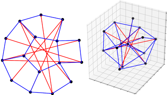
## Diagram: 2D and 3D Network Graph Representations ### Overview The image displays two visualizations of the same underlying network graph structure. On the left is a two-dimensional (2D) planar embedding, and on the right is a three-dimensional (3D) spatial embedding of the same graph. The graph consists of nodes (vertices) connected by edges (links) of two distinct colors, suggesting two different types of relationships or connections. ### Components/Axes * **Left Diagram (2D Graph):** * **Nodes:** 16 black circular points representing vertices. * **Edges:** Lines connecting the nodes. * **Blue Edges:** Form the outer perimeter and some internal connections, creating a polygonal boundary. * **Red Edges:** Create a dense, interconnected web primarily within the interior of the structure. * **Layout:** A force-directed or similar 2D layout designed to minimize edge crossings and show the graph's topology clearly. No coordinate axes or labels are present. * **Right Diagram (3D Graph):** * **Nodes:** The same 16 black points, now positioned in 3D space. * **Edges:** The same set of blue and red connections between nodes. * **Coordinate System:** A 3D Cartesian grid is shown as a wireframe box, providing spatial context. The grid has three visible faces (bottom, left, and back) with faint grid lines. No axis labels, titles, or scale markers are provided. * **Layout:** The graph is embedded in 3D space, which may reveal different structural properties or clusters not as apparent in the 2D view. ### Detailed Analysis * **Node Count:** There are exactly 16 nodes in both representations. * **Edge Color Coding:** * **Blue Edges:** Appear to form a connected outer shell or cycle. In the 2D view, they create a roughly decagonal (10-sided) outer boundary with additional blue connections inside. * **Red Edges:** Form a highly interconnected core. In the 2D view, they create a complex, star-like pattern with many edges crossing the interior. * **Spatial Relationship:** The 3D view on the right is a perspective projection of the graph. The same topological connections (which node is linked to which) are preserved between the two views. The 3D view suggests the graph has depth, with some nodes positioned "behind" others relative to the viewer's perspective. * **Absence of Text:** The image contains no textual labels, titles, legends, axis annotations, or data values. All information is conveyed through the geometric structure and color coding of the graph elements. ### Key Observations 1. **Dual Representation:** The core purpose of the image is to contrast a 2D topological layout with a 3D spatial embedding of an identical network. 2. **Color-Coded Connectivity:** The use of two distinct edge colors (blue and red) strongly implies the graph has two types of edges, which could represent different relationships (e.g., strong vs. weak links, different protocols, physical vs. logical connections). 3. **High Connectivity:** The graph is dense, particularly with red edges, indicating a highly interconnected system rather than a sparse tree or chain structure. 4. **Structural Insight:** The 3D view may be intended to show that the graph is not planar (cannot be drawn in 2D without edges crossing) or to highlight a specific three-dimensional clustering or symmetry. ### Interpretation This image is a technical diagram used in fields like network science, graph theory, computational biology, or computer networking. It serves to visualize the topology and potential spatial organization of a complex system. * **What it Demonstrates:** It shows how the same set of connections can be visualized differently to emphasize different properties. The 2D view (left) is optimal for understanding the pure connectivity and relationships between nodes without the distortion of perspective. The 3D view (right) may model a more realistic physical or abstract spatial arrangement, potentially revealing clusters, hierarchies, or the system's inherent dimensionality. * **Relationship Between Elements:** The nodes are the fundamental entities (e.g., servers, neurons, proteins, people). The colored edges represent specific interactions or pathways between them. The blue edges might form a foundational or backbone network, while the red edges represent a secondary, more complex overlay of interactions. * **Notable Patterns:** The dense red core suggests a "small-world" network property, where most nodes can be reached from any other via a short path. The outer blue shell could indicate a boundary or a different functional layer of the network. The lack of labels focuses the viewer entirely on the structural patterns. * **Purpose:** Such diagrams are used to analyze network robustness, identify central nodes, plan efficient routing, or understand the structural principles of complex systems. The side-by-side comparison is a common method to argue for the necessity of a particular visualization or to study how layout algorithms affect the perception of network structure.

## Network Diagram: 2D and 3D Representation of a Connected System ### Overview The image presents two views of a network diagram: a 2D projection on the left and a 3D perspective on the right. The network consists of **black nodes** (vertices) connected by **red and blue edges** (links). The 3D view is overlaid on a grid background, suggesting spatial orientation. No textual labels, legends, or axis markers are visible in the image. ### Components/Axes - **Nodes**: Black circular points representing entities or data points. - **Edges**: - **Red edges**: Likely denote primary connections or high-priority relationships. - **Blue edges**: May represent secondary or auxiliary connections. - **Views**: - **2D View (Left)**: Flat, planar representation with overlapping edges. - **3D View (Right)**: Perspective projection with depth, showing nodes and edges in a grid-aligned space. ### Detailed Analysis - **Node Distribution**: - Approximately **15–20 nodes** are visible in both views. - Nodes are clustered in the center of the 3D view, with sparser distribution toward the edges. - **Edge Density**: - Red edges dominate the central region, forming dense interconnections. - Blue edges are more peripheral, connecting outer nodes to the core. - **Spatial Grounding**: - The 3D grid provides a reference frame, but no explicit axis labels (X, Y, Z) are visible. - Nodes and edges are evenly distributed across the grid, with no clear positional bias. ### Key Observations 1. **Color Coding**: Red and blue edges are spatially segregated, suggesting a categorical distinction (e.g., priority, type, or direction). 2. **Network Complexity**: The 3D view reveals overlapping edges and nodes, indicating a highly interconnected system. 3. **Missing Metadata**: No legends, axis titles, or numerical data are present to quantify relationships or node attributes. ### Interpretation The diagram likely represents a **complex network system** (e.g., social, technological, or biological) with hierarchical or layered relationships. The red edges may signify core interactions, while blue edges could represent peripheral or auxiliary links. The absence of labels or legends limits quantitative analysis, but the spatial segregation of edge colors implies a structured hierarchy. The 3D perspective emphasizes depth and connectivity, suggesting the system’s multidimensional nature. **Note**: No textual or numerical data is extractable from the image. The analysis is based solely on visual patterns and spatial relationships.