## Diagram: Optimization Process ### Overview The image illustrates an optimization process, likely related to machine learning or a similar field. It shows the iterative steps of updating a parameter θ to reach an optimal value θ*. The diagram uses arrows and equations to represent the update rules and the search for the optimal value. ### Components/Axes * **Nodes:** * θt: Initial parameter value (black dot) * Intermediate point (blue dot) * θ̃t+1: Intermediate parameter value (purple dot) * θ*: Optimal parameter value (black dot) * **Arrows:** * Blue arrow: Represents the gradient descent step. * Purple dashed arrow: Represents the optimization step to find θ̃t+1. * Dashed gray line: Represents the direct path from θt to θ*. * **Equations:** * θt+1 = θt - ηt∇θL̂(θ; πθt)|θ=θt (Blue text, top-left) * θ̃t+1 = arg maxθ J(θ; πθt) = arg minθ L̂(θ; πθt) (Purple text, top-right) ### Detailed Analysis * **Initial State (θt):** The process starts at θt, represented by a black dot on the left. * **Gradient Descent Step (Blue):** A blue arrow originates from θt, indicating a step in the direction of the negative gradient of the loss function L̂. The equation θt+1 = θt - ηt∇θL̂(θ; πθt)|θ=θt describes this update, where ηt is the learning rate and ∇θL̂(θ; πθt) is the gradient of the loss function with respect to θ, evaluated at θt. This step leads to an intermediate blue dot. * **Optimization Step (Purple):** A purple dashed arrow originates from the blue dot and curves upwards to a purple dot labeled θ̃t+1. This represents an optimization step to find the best θ given the current policy πθt. The equation θ̃t+1 = arg maxθ J(θ; πθt) = arg minθ L̂(θ; πθt) describes this step, where J is a reward function and L̂ is a loss function. * **Optimal State (θ*):** A purple dashed arrow originates from θ̃t+1 and curves downwards to the final black dot labeled θ*. This represents the final step in the optimization process, aiming to reach the optimal parameter value θ*. * **Direct Path (Gray):** A dashed gray line connects θt directly to θ*, representing the ideal, but often unattainable, direct path to the optimal value. ### Key Observations * The diagram illustrates an iterative optimization process. * The process involves both gradient descent and a separate optimization step. * The goal is to find the optimal parameter value θ*. ### Interpretation The diagram depicts a two-stage optimization process. The blue arrow represents a gradient descent step, which moves the parameter θ in the direction of decreasing loss. The purple arrow represents a more sophisticated optimization step, which aims to find the best θ given the current policy. This could represent a policy improvement step in reinforcement learning, where the policy is updated to maximize the expected reward. The dashed gray line represents the ideal, but often unattainable, direct path to the optimal value. The diagram highlights the iterative nature of the optimization process and the interplay between gradient descent and policy optimization.

\n ## Diagram: Optimization Path ### Overview The image depicts a visual representation of an optimization process, likely gradient descent, showing the iterative steps towards finding the optimal parameter value (θ*). It combines a graphical illustration of the path taken during optimization with mathematical equations defining the update rule. ### Components/Axes The diagram consists of: * A horizontal axis representing the parameter space, labeled with θ_t on the left and θ^* on the right. * A curved path illustrating the optimization trajectory. * Points along the path, colored differently to indicate the progression of the optimization. * Arrows indicating the direction of the update step. * Mathematical equations describing the update rule and the optimization objective. ### Detailed Analysis or Content Details The equations presented are: 1. θ_t+1 = θ_t - η∇_θL(θ; π_θt) 2. θ_t+1 = argmax_θ J(θ; π_θt) 3. = argmin_θ L(θ; π_θt) Where: * θ_t represents the parameter value at time step t. * θ_t+1 represents the parameter value at the next time step. * η (eta) is the learning rate. * ∇_θL(θ; π_θt) is the gradient of the loss function L with respect to the parameter θ, evaluated at θ_t and given the policy π_θt. * J(θ; π_θt) is the objective function to be maximized. * L(θ; π_θt) is the loss function to be minimized. * π_θt represents the policy at time step t. * θ^* represents the optimal parameter value. The diagram shows the following steps: * **Initial Point:** A black circle at θ_t. * **First Update:** A blue circle connected to the initial point by an arrow, representing the first update step. * **Intermediate Point:** A purple circle representing an intermediate parameter value. * **Final Point:** A black circle at θ^*, indicating the optimal parameter value. * **Optimization Path:** A dashed purple curve connecting the intermediate points, illustrating the overall optimization trajectory. ### Key Observations The diagram illustrates that the optimization process involves iteratively updating the parameter value (θ) by moving in the opposite direction of the gradient of the loss function (∇_θL). The learning rate (η) controls the step size. The goal is to reach the optimal parameter value (θ^*) where the loss function is minimized or the objective function is maximized. The path is not necessarily a straight line, and may involve oscillations or curves as it approaches the optimum. ### Interpretation This diagram visually explains the core concept of gradient-based optimization algorithms. The equations and the graphical representation work together to convey the iterative nature of the process. The diagram suggests that the optimization process starts from an initial parameter value (θ_t) and iteratively updates it based on the gradient of the loss function, eventually converging to the optimal parameter value (θ^*). The choice of learning rate (η) is crucial for the success of the optimization process; a too-large learning rate may cause oscillations or divergence, while a too-small learning rate may lead to slow convergence. The diagram highlights the trade-off between exploration (moving in the direction of the gradient) and exploitation (converging to the optimum). The use of both the mathematical notation and the visual representation makes the concept accessible to a wider audience. The diagram is a simplified representation of a complex process, but it effectively captures the essential elements of gradient-based optimization.

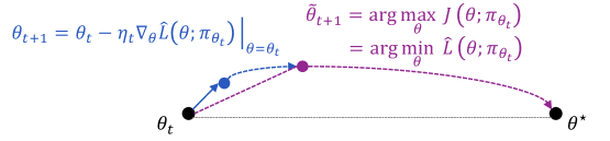
## Diagram: Optimization Process Flow ### Overview The image is a technical diagram illustrating two different optimization update rules in machine learning, visually comparing their trajectories from an initial parameter state (θ_t) toward an optimal state (θ*). It combines mathematical equations with a graphical representation of parameter space movement. ### Components/Axes **Top Section (Equations):** 1. **Left Equation (Blue Text):** `θ_{t+1} = θ_t - η_t ∇_θ L̂(θ; π_{θ_t}) |_{θ=θ_t}` * This is a standard gradient descent update rule. * **Components:** `θ_{t+1}` (updated parameters), `θ_t` (current parameters), `η_t` (learning rate), `∇_θ` (gradient operator), `L̂` (estimated loss function), `π_{θ_t}` (policy parameterized by `θ_t`). 2. **Right Equation (Purple Text):** `θ̃_{t+1} = arg max_θ J(θ; π_{θ_t})` `= arg min_θ L̂(θ; π_{θ_t})` * This defines an alternative update rule that seeks the parameters maximizing an objective `J` (or equivalently, minimizing the estimated loss `L̂`) directly, given the current policy `π_{θ_t}`. * **Components:** `θ̃_{t+1}` (updated parameters via this rule), `arg max_θ`/`arg min_θ` (argument of the maximum/minimum), `J` (objective function). **Bottom Section (Visual Diagram):** * **Points:** * `θ_t`: Black dot, positioned at the bottom-left. Represents the starting parameter state at time `t`. * `θ_{t+1}`: Blue dot, positioned to the right and slightly above `θ_t`. Represents the parameter state after one step of the gradient descent update (left equation). * `θ̃_{t+1}`: Purple dot, positioned further right and higher than `θ_{t+1}`. Represents the parameter state after one step of the `arg max`/`arg min` update (right equation). * `θ*`: Black dot, positioned at the bottom-right. Represents the optimal parameter state. * **Arrows/Paths:** * **Solid Blue Arrow:** Connects `θ_t` to `θ_{t+1}`. Corresponds to the gradient descent update (left equation). * **Dashed Purple Arrow:** Connects `θ_t` to `θ̃_{t+1}`. Corresponds to the `arg max`/`arg min` update (right equation). * **Dotted Black Line:** Connects `θ_t` directly to `θ*`. Represents a hypothetical direct path to the optimum. * **Dashed Purple Arc:** Connects `θ̃_{t+1}` to `θ*`. Suggests a subsequent path from the intermediate point to the optimum. ### Detailed Analysis * **Spatial Grounding & Color Correspondence:** * The **blue** text of the left equation corresponds to the **blue** dot (`θ_{t+1}`) and the **solid blue arrow**. * The **purple** text of the right equation corresponds to the **purple** dot (`θ̃_{t+1}`) and the **dashed purple arrow** and arc. * The **black** dots (`θ_t`, `θ*`) and the **dotted black line** are neutral, representing start and end points. * **Trend Verification:** * The **gradient descent path (blue)** shows a small, incremental step from `θ_t` toward the general direction of `θ*`, but it lands at `θ_{t+1}`, which is not on the direct line to `θ*`. * The **`arg max`/`arg min` path (purple dashed)** shows a larger, more direct leap from `θ_t` to `θ̃_{t+1}`, which is positioned closer to the vertical level of `θ*` and further along the horizontal axis. * The **dotted black line** shows the ideal, straight-line path from start to optimum. ### Key Observations 1. The diagram visually contrasts a local, gradient-based step (blue) with a more global, objective-based step (purple). 2. The point `θ̃_{t+1}` is depicted as being "higher" (potentially indicating a higher objective value `J`) and further along the path to `θ*` than `θ_{t+1}` after a single update. 3. The dashed purple arc from `θ̃_{t+1}` to `θ*` implies that the `arg max` update places the parameters on a more favorable trajectory for reaching the optimum, possibly requiring fewer subsequent steps. ### Interpretation This diagram is likely from a reinforcement learning or optimization theory context. It illustrates a conceptual comparison between two fundamental update strategies: * **Gradient Descent (Blue):** A first-order method that follows the local slope of the loss landscape. It's computationally efficient but can be slow, myopic, and prone to getting stuck in local minima or taking a circuitous path. * **Direct Objective Optimization (Purple):** A method that, at each step, seeks the parameters that would be optimal *if the current policy (π_{θ_t}) were fixed*. This is a more aggressive, "look-ahead" or "policy improvement" step. In algorithms like Trust Region Policy Optimization (TRPO) or Proximal Policy Optimization (PPO), such steps are constrained to ensure stability. The visual metaphor suggests that while the gradient step makes safe, small progress, the direct optimization step makes a more significant leap toward regions of higher reward (or lower loss), potentially leading to faster overall convergence to the optimum `θ*`. The diagram argues for the potential efficiency of the latter approach by showing its intermediate point (`θ̃_{t+1}`) as being qualitatively closer to the goal.

## Diagram: Gradient-Based Optimization Process ### Overview The image depicts a mathematical optimization process involving parameter updates and trajectory visualization. It combines equations describing iterative updates with a graphical representation of the optimization landscape and parameter evolution. ### Components/Axes 1. **Equations**: - Left side: - `θ_{t+1} = θ_t - η_t∇_θL(θ; π_θ_t) |_{θ=θ_t}` (Gradient descent update rule) - `θ̃_{t+1} = arg max_θ J(θ; π_θ_t) = arg min_θ L̃(θ; π_θ_t)` (Optimization objective equivalence) - Right side: - Graph showing parameter space with points θ_t, θ̃_{t+1}, and θ* 2. **Graph Elements**: - **Points**: - θ_t (black dot, starting position) - θ̃_{t+1} (purple dot, next parameter estimate) - θ* (black dot, optimal parameter) - **Arrows**: - Blue arrow: Gradient vector ∇_θL(θ; π_θ_t) pointing from θ_t to θ̃_{t+1} - Purple dashed line: Optimization trajectory from θ_t to θ* - **Axes**: Implicit parameter space axes (no explicit labels) 3. **Color Coding**: - Blue: Gradient direction (∇_θL) - Purple: Optimization trajectory (J(θ) maximization/L̃ minimization) ### Detailed Analysis - **Gradient Descent Update**: - θ_{t+1} is calculated by subtracting the gradient of the loss function L scaled by learning rate η_t from the current parameter θ_t. - The gradient ∇_θL(θ; π_θ_t) is evaluated at the current parameter θ_t. - **Optimization Objective**: - θ̃_{t+1} is determined by maximizing the objective function J(θ; π_θ_t), which is equivalent to minimizing the loss function L̃(θ; π_θ_t). - This represents a dual perspective of the same optimization problem. - **Trajectory Visualization**: - The purple dashed line shows the path from the current parameter θ_t toward the optimal parameter θ*. - The blue gradient vector indicates the direction of steepest ascent for the objective function J. ### Key Observations 1. The gradient vector (blue) points directly toward θ̃_{t+1}, confirming it as the next parameter estimate. 2. The optimization trajectory (purple) curves toward θ*, suggesting convergence to the optimal solution. 3. θ̃_{t+1} lies between θ_t and θ* on the trajectory, indicating iterative progress. 4. The equivalence between maximizing J and minimizing L̃ is visually represented through the shared trajectory. ### Interpretation This diagram illustrates a gradient-based optimization algorithm, likely in machine learning or statistical inference. The process involves: 1. **Parameter Update**: Adjusting θ_t using gradient descent to compute θ̃_{t+1}. 2. **Objective Optimization**: Simultaneously framing the problem as maximizing J or minimizing L̃. 3. **Convergence**: The trajectory (purple line) demonstrates movement toward the optimal parameter θ*. The visualization emphasizes the relationship between gradient direction and optimization trajectory, showing how iterative updates navigate the parameter space toward the optimal solution. The equivalence between the maximization and minimization formulations highlights the duality in optimization problems, where different objective formulations can lead to the same parameter updates.