\n
## Diagram: Optimization Path
### Overview
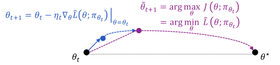
The image depicts a visual representation of an optimization process, likely gradient descent, showing the iterative steps towards finding the optimal parameter value (θ*). It combines a graphical illustration of the path taken during optimization with mathematical equations defining the update rule.
### Components/Axes
The diagram consists of:
* A horizontal axis representing the parameter space, labeled with θ<sub>t</sub> on the left and θ<sup>*</sup> on the right.
* A curved path illustrating the optimization trajectory.
* Points along the path, colored differently to indicate the progression of the optimization.
* Arrows indicating the direction of the update step.
* Mathematical equations describing the update rule and the optimization objective.
### Detailed Analysis or Content Details
The equations presented are:
1. θ<sub>t+1</sub> = θ<sub>t</sub> - η∇<sub>θ</sub>L(θ; π<sub>θt</sub>)
2. θ<sub>t+1</sub> = argmax<sub>θ</sub> J(θ; π<sub>θt</sub>)
3. = argmin<sub>θ</sub> L(θ; π<sub>θt</sub>)
Where:
* θ<sub>t</sub> represents the parameter value at time step t.
* θ<sub>t+1</sub> represents the parameter value at the next time step.
* η (eta) is the learning rate.
* ∇<sub>θ</sub>L(θ; π<sub>θt</sub>) is the gradient of the loss function L with respect to the parameter θ, evaluated at θ<sub>t</sub> and given the policy π<sub>θt</sub>.
* J(θ; π<sub>θt</sub>) is the objective function to be maximized.
* L(θ; π<sub>θt</sub>) is the loss function to be minimized.
* π<sub>θt</sub> represents the policy at time step t.
* θ<sup>*</sup> represents the optimal parameter value.
The diagram shows the following steps:
* **Initial Point:** A black circle at θ<sub>t</sub>.
* **First Update:** A blue circle connected to the initial point by an arrow, representing the first update step.
* **Intermediate Point:** A purple circle representing an intermediate parameter value.
* **Final Point:** A black circle at θ<sup>*</sup>, indicating the optimal parameter value.
* **Optimization Path:** A dashed purple curve connecting the intermediate points, illustrating the overall optimization trajectory.
### Key Observations
The diagram illustrates that the optimization process involves iteratively updating the parameter value (θ) by moving in the opposite direction of the gradient of the loss function (∇<sub>θ</sub>L). The learning rate (η) controls the step size. The goal is to reach the optimal parameter value (θ<sup>*</sup>) where the loss function is minimized or the objective function is maximized. The path is not necessarily a straight line, and may involve oscillations or curves as it approaches the optimum.
### Interpretation
This diagram visually explains the core concept of gradient-based optimization algorithms. The equations and the graphical representation work together to convey the iterative nature of the process. The diagram suggests that the optimization process starts from an initial parameter value (θ<sub>t</sub>) and iteratively updates it based on the gradient of the loss function, eventually converging to the optimal parameter value (θ<sup>*</sup>). The choice of learning rate (η) is crucial for the success of the optimization process; a too-large learning rate may cause oscillations or divergence, while a too-small learning rate may lead to slow convergence. The diagram highlights the trade-off between exploration (moving in the direction of the gradient) and exploitation (converging to the optimum). The use of both the mathematical notation and the visual representation makes the concept accessible to a wider audience. The diagram is a simplified representation of a complex process, but it effectively captures the essential elements of gradient-based optimization.